Note
Go to the end to download the full example code.
Inria Raweb dataset with Pipeline API
In this example we will process Inria Raweb dataset using Pipeline API.
The pipeline will comprise of the following steps:
extract entities
use Latent Semantic Analysis (LSA) to generate n-dimensional vector representation of the entities
use Uniform Manifold Approximation and Projection (UMAP) to project those entities in 2 dimensions
use KMeans clustering to cluster entities
find their nearest neighbors.
All files necessary to run Inria Raweb pipeline can be downloaded from https://zenodo.org/record/7970984.
Create Inria Raweb Dataset
We will first create Dataset for Inria Raweb.
The CSV file rawebdf.csv contains the dataset data.
from cartodata.pipeline.datasets import CSVDataset  # noqa
from pathlib import Path # noqa

ROOT_DIR = Path.cwd().parent
# The directory where files necessary to load dataset columns reside
INPUT_DIR = ROOT_DIR / "datas"
# The directory where the generated dump files will be saved
TOP_DIR = ROOT_DIR / "dumps"

dataset = CSVDataset("inriaraweb", input_dir=INPUT_DIR, version="1.0.0", filename="raweb.csv",
                     fileurl="https://zenodo.org/record/7970984/files/raweb.csv")

dataset.df.head()
Downloading data from https://zenodo.org/records/7970984/files/raweb.csv (154.9 MB)


file_sizes:   0%|                                    | 0.00/162M [00:00<?, ?B/s]
file_sizes:   2%|▌                          | 3.11M/162M [00:00<00:05, 29.6MB/s]
file_sizes:   4%|█                          | 6.26M/162M [00:00<00:06, 25.1MB/s]
file_sizes:   7%|█▉                         | 12.0M/162M [00:00<00:04, 36.2MB/s]
file_sizes:  10%|██▋                        | 16.2M/162M [00:00<00:03, 38.2MB/s]
file_sizes:  13%|███▍                       | 20.4M/162M [00:00<00:04, 35.1MB/s]
file_sizes:  15%|████                       | 24.6M/162M [00:00<00:03, 34.5MB/s]
file_sizes:  19%|█████▏                     | 30.9M/162M [00:00<00:03, 40.5MB/s]
file_sizes:  24%|██████▌                    | 39.3M/162M [00:00<00:02, 51.8MB/s]
file_sizes:  29%|███████▉                   | 47.7M/162M [00:01<00:02, 54.1MB/s]
file_sizes:  36%|█████████▋                 | 58.2M/162M [00:01<00:01, 66.5MB/s]
file_sizes:  41%|███████████                | 66.6M/162M [00:01<00:01, 65.1MB/s]
file_sizes:  47%|████████████▊              | 77.0M/162M [00:01<00:01, 73.9MB/s]
file_sizes:  53%|██████████████▏            | 85.4M/162M [00:01<00:01, 74.8MB/s]
file_sizes:  59%|███████████████▉           | 95.9M/162M [00:01<00:00, 74.4MB/s]
file_sizes:  66%|██████████████████▎         | 106M/162M [00:01<00:00, 77.5MB/s]
file_sizes:  71%|███████████████████▊        | 115M/162M [00:01<00:00, 77.2MB/s]
file_sizes:  77%|█████████████████████▌      | 125M/162M [00:02<00:00, 84.1MB/s]
file_sizes:  84%|███████████████████████▍    | 136M/162M [00:02<00:00, 80.4MB/s]
file_sizes:  89%|████████████████████████▊   | 144M/162M [00:02<00:00, 74.9MB/s]
file_sizes:  97%|███████████████████████████ | 157M/162M [00:02<00:00, 84.8MB/s]
file_sizes: 100%|████████████████████████████| 162M/162M [00:02<00:00, 66.5MB/s]
Successfully downloaded file to dumps/inriaraweb/1.0.0/raweb.csv
/builds/2mk6rsew/0/hgozukan/cartolabe-data/cartodata/pipeline/datasets.py:537: DtypeWarning: Columns (7) have mixed types. Specify dtype option on import or set low_memory=False.
  return pd.read_csv(raw_file, **self.kwargs)
The dataframe that we just read consists of 118455 rows.
dataset.df.shape[0]
118455
And has name, team, teamyear, year, center, theme, text and keywords as columns.
print(*dataset.df.columns, sep="\n")
name
team
teamyear
year
center
theme
text
keywords
Now we should define our entities and set the column names corresponding to those entities from the data file. We have 7 entities:
———|-------------| | rawebpart | name | | teams | teams | | cwords | text | | teamyear | teamyear | | center | center | | theme | theme | | words | text |
Cartolabe provides 4 types of columns:
IdentityColumn: The entity of this column represents the main entity of the dataset. The column data corresponding to the entity in the file should contain a single value and this value should be unique among column values. There can only be one IdentityColumn in the dataset.
CSColumn: The entity of this column type is related to the main entity, and can contain single or comma separated values.
CorpusColumn: The entity of this column type is the corpus related to the main entity. This can be a combination of multiple columns in the file. It uses a modified version of CountVectorizer(https://scikit-learn.org/stable/modules/generated/sklearn.feature_extraction.text.CountVectorizer.html#sklearn.feature_extraction.text.CountVectorizer).
TfidfCorpusColumn: The entity of this column type is the corpus related to the main entity. This can be a combination of multiple columns in the file or can contain filepath from which to read the text corpus. It uses TfidfVectorizer (https://scikit-learn.org/stable/modules/generated/sklearn.feature_extraction.text.TfidfVectorizer.html).
To define the columns we will need additinal files, stopwords_raweb.txt and inriavocab.csv. We can download them from Zenodo and save under ../datas directory.
from download import download  # noqa

stopwords_url = "https://zenodo.org/record/7970984/files/stopwords_raweb.txt"
vocab_url = "https://zenodo.org/record/7970984/files/inriavocab.csv"

download(stopwords_url, INPUT_DIR / "stopwords_raweb.txt", kind='file',
         progressbar=True, replace=False)

download(vocab_url, INPUT_DIR / "inriavocab.csv", kind='file',
         progressbar=True, replace=False)
Downloading data from https://zenodo.org/records/7970984/files/stopwords_raweb.txt (5 kB)


file_sizes:   0%|                                   | 0.00/4.85k [00:00<?, ?B/s]
file_sizes: 100%|██████████████████████████| 4.85k/4.85k [00:00<00:00, 5.03MB/s]
Successfully downloaded file to /builds/2mk6rsew/0/hgozukan/cartolabe-data/datas/stopwords_raweb.txt
Downloading data from https://zenodo.org/records/7970984/files/inriavocab.csv (1.1 MB)


file_sizes:   0%|                                   | 0.00/1.18M [00:00<?, ?B/s]
file_sizes: 100%|██████████████████████████| 1.18M/1.18M [00:00<00:00, 19.7MB/s]
Successfully downloaded file to /builds/2mk6rsew/0/hgozukan/cartolabe-data/datas/inriavocab.csv

'/builds/2mk6rsew/0/hgozukan/cartolabe-data/datas/inriavocab.csv'
In this dataset, rawebpart is our main entity. We will define it as IdentityColumn:
from cartodata.pipeline.columns import IdentityColumn, CSColumn, CorpusColumn  # noqa


rawebpart_column = IdentityColumn(nature="rawebpart", column_name="name")

teams_column = CSColumn(nature="teams", column_name="team",
                        filter_min_score=4)

cwords_column = CorpusColumn(nature="cwords", column_names=["text"],
                             stopwords="stopwords_raweb.txt", nb_grams=4,
                             min_df=25, max_df=0.05, normalize=True,
                             vocabulary="inriavocab.csv")

teamyear_column = CSColumn(nature="teamyear", column_name="teamyear",
                           filter_min_score=4)

center_column = CSColumn(nature="center", column_name="center", separator=";")

theme_column = CSColumn(nature="theme", column_name="theme", separator=";",
                        filter_nan=True)

words_column = CorpusColumn(nature="words", column_names=["text"],
                            stopwords="stopwords_raweb.txt", nb_grams=4,
                            min_df=25, max_df=0.1, normalize=True)
Now we are going to set the columns of the dataset:
dataset.set_columns([rawebpart_column, teams_column, cwords_column, teamyear_column,
                     center_column, theme_column, words_column])
We can set the columns in any order that we prefer. We will set the first entity as identity entity and the last entity as the corpus. If we set the entities in a different order, the Dataset will put the main entity as first.
The dataset for Inria Raweb data is ready. Now we will create and run our pipeline. For this pipeline, we will:
run LSA projection -> N-dimesional
run UMAP projection -> 2D
cluster entities
find nearest neighbors
Create and run pipeline
We will first create a pipeline with the dataset.
from cartodata.pipeline.common import Pipeline  # noqa

pipeline = Pipeline(dataset=dataset, top_dir=TOP_DIR, input_dir=INPUT_DIR)
The workflow generates the natures from dataset columns.
pipeline.natures
['rawebpart', 'teams', 'cwords', 'teamyear', 'center', 'theme', 'words']
Creating correspondance matrices for each entity type
Now we want to extract matrices that will map the correspondance between each name in the dataset and the entities we want to use.
Pipeline has generate_entity_matrices function to generate matrices and scores for each entity (nature) specified for the dataset.
matrices, scores = pipeline.generate_entity_matrices(force=True)
Rawebpart
The first matrix in matrices and Series in scores corresponds to rawebpart.
The type for tout column is IdentityColumn. It generates a matrix that simply maps each row entry to itself.
rawebpart_mat = matrices[0]
rawebpart_mat.shape
(118455, 118455)
Having type IdentityColumn, each item will have score 1.
rawebpart_scores = scores[0]
rawebpart_scores.shape

rawebpart_scores.head()
abs2018_presentation_Overall Objectives (0)                   1.0
abs2018_fondements_Introduction (1)                           1.0
abs2018_fondements_Modeling interfaces and contacts (2)       1.0
abs2018_fondements_Modeling macro-molecular assemblies (3)    1.0
abs2018_fondements_Reconstruction by Data Integration (4)     1.0
dtype: float64
Teams
The second matrix in matrices and score in scores correspond to teams.
The type for teams is CSColumn. It generates a sparce matrix where rows correspond to rows and columns corresponds to the teams obtained by separating comma separated values.
teams_mat = matrices[1]
teams_mat.shape

teams_scores = scores[1]
teams_scores.head()

teams_scores.shape
(469,)
Cwords
The third matrix in matrices and score in scores correspond to cwords.
The type for cwords column is CorpusColumn. It uses text column in the dataset, and then extracts n-grams from that corpus using a fixed vocabulary ../datas/inriavocab.csv. Finally it generates a sparce matrix where rows correspond to each entry in the dataset and columns corresponds to n-grams.
cwords_mat = matrices[2]
cwords_mat.shape

cwords_scores = scores[2]
cwords_scores.head()
abandon        32
abbreviated    32
abdalla        49
abdominal      50
abelian        86
dtype: int64
Teamyear
The fourth matrix in matrices and score in scores correspond to teamyear.
The type for teamyear is CSColumn. It generates a sparce matrix where rows correspond to rows and columns corresponds to the team year values obtained by separating comma separated values.
teamyear_mat = matrices[3]
teamyear_mat.shape

teamyear_scores = scores[3]
teamyear_scores.head()
abs2018       29
acumes2018    46
agora2018     43
airsea2018    49
alice2018     26
dtype: int64
Center
The fifth matrix in matrices and score in scores correspond to center.
The type for center is CSColumn. It generates a sparce matrix where rows correspond to rows and columns corresponds to the centers.
center_mat = matrices[4]
center_mat.shape

center_scores = scores[4]
center_scores.head()
Sophia Antipolis - Méditerranée    20884
Grenoble - Rhône-Alpes             19230
Nancy - Grand Est                  12171
Paris                               4595
Bordeaux - Sud-Ouest                8728
dtype: int64
Theme
The sixth matrix in matrices and score in scores correspond to theme.
The type for theme is CSColumn. It generates a sparce matrix where rows correspond to rows and columns corresponds to the theme obtained by separating comma separated values.
theme_mat = matrices[5]
theme_mat.shape

theme_scores = scores[5]
theme_scores.head()
Computational Sciences for Biology, Medicine and the Environment    18003
Applied Mathematics, Computation and Simulation                     16704
Networks, Systems and Services, Distributed Computing               19866
Perception, Cognition, Interaction                                  22013
Algorithmics, Programming, Software and Architecture                19166
dtype: int64
Words
The seventh matrix in matrices and score in scores correspond to words.
The type for words column is CorpusColumn. It creates a corpus merging multiple text columns in the dataset, and then extracts n-grams from that corpus. Finally it generates a sparce matrix where rows correspond to articles and columns corresponds to n-grams.
words_mat = matrices[6]
words_mat.shape
(118455, 56532)
Here we see that there are 56532 distinct n-grams.
The series, which we named words_scores, contains the list of n-grams with a score that is equal to the number of rows that this value was mapped within the words_mat matrix.
words_scores = scores[6]
words_scores.head(10)
015879     93
10000     159
100ms      27
150000     27
1960s      43
1970s      74
1980s      67
1990s      98
20000      39
2000s      47
dtype: int64
Dimension reduction
One way to see the matrices that we created is as coordinates in the space of all articles. What we want to do is to reduce the dimension of this space to make it easier to work with and see.
LSA projection
We’ll start by using the LSA (Latent Semantic Analysis) technique to reduce the number of rows in our data.
from cartodata.pipeline.projectionnd import LSAProjection  # noqa

num_dim = 100

lsa_projection = LSAProjection(num_dim)
pipeline.set_projection_nd(lsa_projection)
Now we can run LSA projection on the matrices.
In our matrices we have 2 columns generated from given corpus; cwords and words. When we create the dataset and set it columns, the dataset sets the index for corpus column as corpus_index. When there are more then one columns of type cartodata.pipeline.columns.CorpusColumn, the index of the final one is set as corpus_index. In our case 6.
We would like to use cwords column as corpus column for LSA projection. So before running the projection, we should set the corpus_index.
pipeline.dataset.corpus_index = 2

""
matrices_nD = pipeline.do_projection_nD(matrices, force=True)

for nature, matrix in zip(pipeline.natures, matrices_nD):
    print(f"{nature}  -------------   {matrix.shape}")
rawebpart  -------------   (100, 118455)
teams  -------------   (100, 469)
cwords  -------------   (100, 29348)
teamyear  -------------   (100, 2715)
center  -------------   (100, 10)
theme  -------------   (100, 5)
words  -------------   (100, 56532)
We have 100 rows for each entity.
This makes it easier to work with them for clustering or nearest neighbors tasks, but we also want to project them on a 2D space to be able to map them.
UMAP projection
The UMAP (Uniform Manifold Approximation and Projection) is a dimension reduction technique that can be used for visualisation similarly to t-SNE.
We use this algorithm to project our matrices in 2 dimensions.
from cartodata.pipeline.projection2d import UMAPProjection  # noqa


umap_projection = UMAPProjection(n_neighbors=10, min_dist=0.1)

pipeline.set_projection_2d(umap_projection)
Now we can run UMAP projection on the LSA matrices.
matrices_2D = pipeline.do_projection_2D(force=True)
Now that we have 2D coordinates for our points, we can try to plot them to get a feel of the data’s shape.
labels = tuple(pipeline.natures)
colors = ['darkgreen', 'red', 'cyan', 'navy',
          'peru', 'gold', 'pink', 'cornflowerblue']

fig, ax = pipeline.plot_map(matrices_2D, labels, colors)

The plot above, as we don’t have labels for the points, doesn’t make much sense as is. But we can see that the data shows some clusters which we could try to identify.
Clustering
In order to identify clusters, we use the KMeans clustering technique on the articles. We’ll also try to label these clusters by selecting the most frequent words that appear in each cluster’s articles.
from cartodata.pipeline.clustering import KMeansClustering # noqa
level of clusters, hl: high level, ml: medium level, ll: low level
cluster_natures = ["hl_clusters", "ml_clusters", "ll_clusters", "vll_clusters"]

kmeans_clustering = KMeansClustering(
    n=8, base_factor=3, natures=cluster_natures)

pipeline.set_clustering(kmeans_clustering)
Now we can run clustering on the matrices.
(clus_nD, clus_2D, clus_scores, cluster_labels,
cluster_eval_pos, cluster_eval_neg) = pipeline.do_clustering()
As we have specified two levels of clustering, the returned lists wil have two values.
len(clus_2D)
4
We will now display two levels of clusters in separate plots, we will start with high level clusters:
clus_scores_hl = clus_scores[0]
clus_mat_hl = clus_2D[0]


fig_hl, ax_hl = pipeline.plot_map(matrices_2D, labels, colors,
                                  title="Inria Raweb Dataset High Level Clusters",
                                  annotations=clus_scores_hl.index,
                                  annotation_mat=clus_mat_hl)
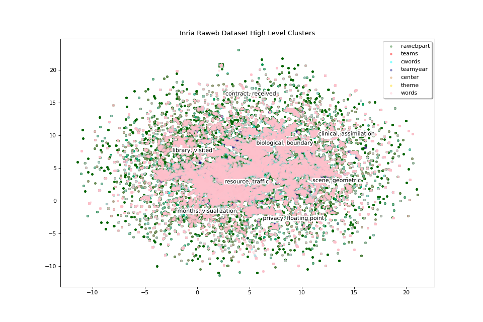
The 8 high level clusters that we created give us a general idea of what the big clusters of data contain.
With medium level clusters we have a finer level of detail:
clus_scores_ml = clus_scores[1]
clus_mat_ml = clus_2D[1]

fig_ml, ax_ml = pipeline.plot_map(matrices_2D, labels, colors,
                                  title="Inria Raweb Dataset Medium Level Clusters",
                                  annotations=clus_scores_ml.index,
                                  annotation_mat=clus_mat_ml)
""
pipeline.save_plot(fig_hl, "inriaraweb_hl_clusters.png")
pipeline.save_plot(fig_ml, "inriaraweb_ml_clusters.png")


for file in pipeline.top_dir.glob("*.png"):
    print(file)
Nearest neighbors
One more thing which could be useful to appreciate the quality of our data would be to get each point’s nearest neighbors.
Finding nearest neighbors is a common task with various algorithms aiming to solve it. The find_neighbors method uses one of these algorithms to find the nearest points of all entities. It takes an optional weight parameter to tweak the distance calculation to select points that have a higher score but are maybe a bit farther instead of just selecting the closest neighbors.
from cartodata.pipeline.neighbors import AllNeighbors  # noqa

n_neighbors = 10
weights = [0, 0, 0, 0, 0, 0, 0.3]

neighboring = AllNeighbors(n_neighbors=n_neighbors, power_scores=weights)

pipeline.set_neighboring(neighboring)

pipeline.find_neighbors()
Export file using exporter
We can now export the data. To export the data, we need to configure the exporter.
The exported data will be the points extracted from the dataset corresponding to the entities that we have defined.
In the export file, we will have the following columns for each point:
———|-------------| | nature | one of tout, prop, question, words, theme, avispositif, avisnegatif, gdprop | | label | point’s label | | score | point’s score | | rank | point’s rank | | x | point’s x location on the map | | y | point’s y location on the map | | nn_rawebpart | neighboring entries to this point | | nn_teams | neighboring props to this point | | nn_cwords | neighboring questions to this point | | nn_teamyear | neighboring words to this point | | nn_lab | neighboring themes to this point | | nn_theme | neighboring avispositifs to this point | | nn_words | neighboring avisnegatifs to this point |
we will call pipeline.export function. It will create export.feather file and save under pipeline.top_dir.
pipeline.export()
Let’s display the contents of the file.
import pandas as pd  # noqa

df = pd.read_feather(pipeline.working_dir / "export.feather")
df.head()
This is a basic export file. For each point, we can add additional columns.
from cartodata.pipeline.exporting import (
    ExportNature, MetadataColumn
)  # noqa


meta_year_article = MetadataColumn(column="year", as_column="year",
                                   func="x.astype(str)")

ex_rawebpart = ExportNature(key="rawebpart",
                            refs=["center", "teams",
                                  "cwords", "theme", "words"],
                            add_metadata=[meta_year_article])

ex_teams = ExportNature(key="teams",
                        refs=["center", "cwords", "theme", "words"])

ex_teamyear = ExportNature(key="teamyear",
                           refs=["center", "teams", "cwords", "theme", "words"])

""
pipeline.export(export_natures=[ex_rawebpart, ex_teams, ex_teamyear])

""
df = pd.read_feather(pipeline.working_dir / "export.feather")
df.head(5)

""
df[df.nature == "rawebpart"].head(1)

""
df[df.nature == "teams"].head(1)

""
df[df.nature == "teamyear"].head(5)
Total running time of the script: (20 minutes 46.555 seconds)