Note
Go to the end to download the full example code.
Extracting and processing LISN data for Cartolabe with Aligned UMAP
(LSA projection)
In this example, we will:
extract entities (authors, articles, labs, words) from a collection of scientific articles
project those entities in 2 dimensions using aligned UMAP
cluster them
find their nearest neighbors.
This example uses 6 datasets containing articles from HAL (https://hal.archives-ouvertes.fr/) published by authors from LISN (Laboratoire Interdisciplinaire des Sciences du Numérique). Each dataset contains cumulative data starting from 2010-2012 to 2010-2022 (inclusive).
Using aligned UMAP will help us align UMAP embeddings for consecutive datasets.
# %matplotlib widget
Download data
We will start by downloading 6 datasets from HAL.
from cartodata.scraping import scrape_hal, process_domain_column   # noqa
import os   # noqa


def fetch_data(from_year, to_year, struct_ids, struct='hal'):
    """
    Fetch scientific publications of struct from HAL.
    """

    filename = f"../datas/{struct.lower()}_{from_year}_{to_year - 1}.csv"

    if os.path.exists(filename):
        return

    filters = {}

    if struct:
        filters['structId_i'] = struct_ids
    years = range(from_year, to_year)
    df = scrape_hal(struct, filters, years, cool_down=2)
    process_domain_column(df)

    # Save the dataframe into a csv file
    df.to_csv(filename)
    return df


# Fetch LRI data from year 2010 to 2022 inclusive
for i in range(2, 14, 2):
    fetch_data(2010, 2011+i, "(1050003 2544)", 'lisn')
Load data
Now we will load each downloaded dataset to a dataframe.
import pandas as pd   # noqa


def load_data(from_year, total, struct):
    dataframes = []

    for i in range(total):
        file_name = f"../datas/{struct.lower()}_{from_year}_{from_year + ( 2 + 2 * i)}.csv"
        print(file_name)
        df = pd.read_csv(file_name, index_col=0)

        dataframes.append(df)

    return dataframes


dataframes = load_data(2010, 6, "lisn")
dataframes[0].head()
../datas/lisn_2010_2012.csv
../datas/lisn_2010_2014.csv
../datas/lisn_2010_2016.csv
../datas/lisn_2010_2018.csv
../datas/lisn_2010_2020.csv
../datas/lisn_2010_2022.csv
We can list the total number of articles starting from 2010 to a certain year.
for i in range(6):
    print(f"{2010 + (i*2) + 2} => {dataframes[i].shape[0]}")
2012 => 765
2014 => 1361
2016 => 1983
2018 => 2514
2020 => 2945
2022 => 2987
Creating correspondance matrices for each entity type
From this table of articles, we want to extract matrices that will map the correspondance between these articles and the entities we want to use.
from cartodata.loading import load_comma_separated_column  # noqa
from cartodata.loading import load_identity_column  # noqa


def create_correspondance_matrices(func, dataframes, column_name):
    matrices = []
    scores = []

    for i in range(len(dataframes)):
        mat, score = func(dataframes[i], column_name)
        matrices.append(mat)
        scores.append(score)

    return matrices, scores
The load_comma_separated_column function takes in a dataframe and the name of a column and returns two objects:
a sparse matrix
a pandas Series
Each column of the sparse matrix, corresponds to the entity specified by column_name and each row corresponds to an article.
Labs
Similarly, we can create matrices for the labs by simply passing the structAcronym_s column to the function.
matrices_labs, scores_labs = create_correspondance_matrices(
    load_comma_separated_column, dataframes, 'structAcronym_s')
We can see the number of (articles, labs) for each year:
for i in range(len(matrices_labs)):
    print(f"{2010 + (i*2) + 2} => {matrices_labs[i].shape}")
2012 => (765, 602)
2014 => (1361, 838)
2016 => (1983, 1041)
2018 => (2514, 1254)
2020 => (2945, 1426)
2022 => (2987, 1447)
Let’s have a look at the number of articles per author for each year:
df_scores_labs = pd.concat(scores_labs, axis=1).reset_index().rename(
    columns={i: f"{2010 + (i*2) + 2}" for i in range(10)}
)

df_scores_labs.head(20)

""
df_scores_labs.describe()
Filtering low score entities
A lot of the authors and labs that we just extracted from the dataframe have a very low score, which means they’re only linked to one or two articles. To improve the quality of our data, we’ll filter the entities by removing those that appear less than certain number of times.
from cartodata.operations import filter_min_score  # noqa


def filter_low_score(matrices, scores, count, entity):

    filtered_matrices = []
    filtered_scores = []

    for i, (matrix, score) in enumerate(zip(matrices, scores)):
        before = len(score)
        filtered_mat, filtered_score = filter_min_score(matrix, score, count)

        filtered_matrices.append(filtered_mat)
        filtered_scores.append(filtered_score)

        print(f'Removed {before - len(filtered_score)} {entity}s with less than ' +
              f'{count} articles from a total of {before} {entity}s.')

        print(f'Working with {len(filtered_score)} {entity} for year {2010 + (i*2) + 2}.\n')

    return filtered_matrices, filtered_scores
Authors
We will remove the authors with less than 5 publications.
auth_pub_count = 5

filtered_auth_matrices, filtered_auth_scores = filter_low_score(
    matrices_auth, scores_auth, auth_pub_count, "author")
Removed 1578 authors with less than 5 articles from a total of 1666 authors.
Working with 88 author for year 2012.

Removed 2179 authors with less than 5 articles from a total of 2338 authors.
Working with 159 author for year 2014.

Removed 2887 authors with less than 5 articles from a total of 3135 authors.
Working with 248 author for year 2016.

Removed 3566 authors with less than 5 articles from a total of 3882 authors.
Working with 316 author for year 2018.

Removed 4168 authors with less than 5 articles from a total of 4554 authors.
Working with 386 author for year 2020.

Removed 4258 authors with less than 5 articles from a total of 4652 authors.
Working with 394 author for year 2022.
Labs
We will remove the labs with less than 20 publications.
lab_pub_count = 20

filtered_lab_matrices, filtered_lab_scores = filter_low_score(
    matrices_labs, scores_labs, lab_pub_count, "labs")
Removed 566 labss with less than 20 articles from a total of 602 labss.
Working with 36 labs for year 2012.

Removed 762 labss with less than 20 articles from a total of 838 labss.
Working with 76 labs for year 2014.

Removed 938 labss with less than 20 articles from a total of 1041 labss.
Working with 103 labs for year 2016.

Removed 1131 labss with less than 20 articles from a total of 1254 labss.
Working with 123 labs for year 2018.

Removed 1286 labss with less than 20 articles from a total of 1426 labss.
Working with 140 labs for year 2020.

Removed 1305 labss with less than 20 articles from a total of 1447 labss.
Working with 142 labs for year 2022.
Words
For the words, it’s a bit trickier because we want to extract n-grams (groups of n terms) instead of just comma separated values. We’ll call the load_text_column which uses scikit-learn’s CountVectorizer <https://scikit-learn.org/stable/modules/generated/sklearn.feature_extraction.text.CountVectorizer.html>_ to create a vocabulary and map the tokens.
from cartodata.loading import load_text_column  # noqa
from sklearn.feature_extraction import text as sktxt  # noqa
from cartodata.operations import normalize_tfidf  # noqa


def process_words(dataframes, stopwords):

    words_matrices = []
    words_scores = []

    for df in dataframes:
        df['text'] = df['en_abstract_s'] + ' ' \
            + df['en_keyword_s'].astype(str) + ' ' \
            + df['en_title_s'].astype(str) + ' ' \
            + df['en_domainAllCodeLabel_fs'].astype(str)

        words_mat, words_score = load_text_column(df['text'],
                                                  4,
                                                  10,
                                                  0.05,
                                                  stopwords=stopwords)
        # apply term-frequency times inverse document-frequency normalization
        words_mat = normalize_tfidf(words_mat)

        words_matrices.append(words_mat)
        words_scores.append(words_score)

    return words_matrices, words_scores


with open('../datas/stopwords.txt', 'r') as stop_file:
    stopwords = sktxt.ENGLISH_STOP_WORDS.union(
        set(stop_file.read().splitlines()))

    words_matrices, words_scores = process_words(dataframes, stopwords)
We can list number of terms per article for each year:
for i in range(len(words_matrices)):
    print(f"{2010 + (i*2) + 2} => {words_matrices[i].shape}")
2012 => (765, 1015)
2014 => (1361, 1801)
2016 => (1983, 2483)
2018 => (2514, 3045)
2020 => (2945, 3512)
2022 => (2987, 3560)
Articles
Finally, we need to create a matrix that simply maps each article to itself.
matrices_article, scores_article = create_correspondance_matrices(
    load_identity_column, dataframes, 'en_title_s')

""
for i in range(len(matrices_article)):
    print(f"{2010 + (i*2) + 2} => {matrices_article[i].shape}")
2012 => (765, 765)
2014 => (1361, 1361)
2016 => (1983, 1983)
2018 => (2514, 2514)
2020 => (2945, 2945)
2022 => (2987, 2987)
Dimension reduction
One way to see the matrices that we created is as coordinates in the space of all articles. What we want to do is to reduce the dimension of this space to make it easier to work with and see.
LSA projection
We’ll start by using the LSA (Latent Semantic Analysis) technique to identify keywords in our data and thus reduce the number of rows in our matrices. The lsa_projection method takes three arguments:
the number of dimensions you want to keep
the matrix of documents/words frequency
a list of matrices to project
It returns a list of the same length containing the matrices projected in the latent space.
We also apply an l2 normalization to each feature of the projected matrices.
from cartodata.projection import lsa_projection  # noqa
from cartodata.operations import normalize_l2  # noqa

dimensions = [12, 12, 14, 16, 20, 20]


def run_lsa_projection(articles_matrices, auth_matrices, words_matrices,
                       lab_matrices, dimensions):
    lsa_matrices = []

    for articles_mat, auth_mat, words_mat, labs_mat, dim in zip(
        articles_matrices, auth_matrices, words_matrices, lab_matrices, dimensions
    ):

        lsa_mat = lsa_projection(
            dim, words_mat, [articles_mat, auth_mat, words_mat, labs_mat]
        )
        lsa_mat = list(map(normalize_l2, lsa_mat))

        lsa_matrices.append(lsa_mat)

    return lsa_matrices


lsa_matrices = run_lsa_projection(matrices_article, filtered_auth_matrices,
                                  words_matrices, filtered_lab_matrices,
                                  dimensions)
List (number_of_articles, dimensions) per year:
for i in range(len(lsa_matrices)):
    print(f"{2010 + (i*2) + 2} => {lsa_matrices[i][0].shape}")
2012 => (12, 765)
2014 => (12, 1361)
2016 => (14, 1983)
2018 => (16, 2514)
2020 => (20, 2945)
2022 => (20, 2987)
List (number_of_authors, dimensions) per year:
for i in range(len(lsa_matrices)):
    print(f"{2010 + (i*2) + 2} => {lsa_matrices[i][1].shape}")
2012 => (12, 88)
2014 => (12, 159)
2016 => (14, 248)
2018 => (16, 316)
2020 => (20, 386)
2022 => (20, 394)
List (number_of_words, dimensions) per year:
for i in range(len(lsa_matrices)):
    print(f"{2010 + (i*2) + 2} => {lsa_matrices[i][2].shape}")
2012 => (12, 1015)
2014 => (12, 1801)
2016 => (14, 2483)
2018 => (16, 3045)
2020 => (20, 3512)
2022 => (20, 3560)
List (number_of_labs, dimensions) per year:
for i in range(len(lsa_matrices)):
    print(f"{2010 + (i*2) + 2} => {lsa_matrices[i][3].shape}")
2012 => (12, 36)
2014 => (12, 76)
2016 => (14, 103)
2018 => (16, 123)
2020 => (20, 140)
2022 => (20, 142)
Aligned UMAP projection
To use aligned UMAP, we need to create relations between each consecutive dataset that maps each entity index (article, author, word, lab) in one dataset to corresponding entity index in the following dataset.
We will also create color mappings to view each entity in consecutive maps with the same color.
import numpy as np  # noqa


def make_relation(from_df, to_df):
    # create a new dataframe with index from from_df, and values as integers
    # starting from 0 to the length of from_df
    left = pd.DataFrame(data=np.arange(len(from_df)), index=from_df.index)

    # create a new dataframe with index from to_df, and values as integers
    # starting from 0 to the length of to_df
    right = pd.DataFrame(data=np.arange(len(to_df)), index=to_df.index)

    # merge left and right dataframes on the intersection of keys of both
    # dataframes preserving the order of left keys
    merge = pd.merge(left, right, how="inner",
                     left_index=True, right_index=True)

    return dict(merge.values)


def generate_relations(filtered_scores):

    relations = []

    for i in range(len(filtered_scores) - 1):
        relation = make_relation(filtered_scores[i], filtered_scores[i+1])

        relations.append(relation)

    return relations


def generate_colors(filtered_scores):

    colors = []

    for i in range(len(filtered_scores)):
        color = make_relation(filtered_scores[i], filtered_scores[-1])

        colors.append(color)

    return colors


def concat_scores(scores_article, scores_auth, scores_word, scores_lab):
    """Concatenates article, auth, words and labs score for each year and
       returns the concatenated frames in a list.
    """
    concatenated_scores = []

    for score_article, score_auth, score_word, score_lab in zip(
        scores_article, scores_auth, scores_word, scores_lab
    ):
        concatenated_scores.append(
            pd.concat([score_article, score_auth, score_word, score_lab]))

    return concatenated_scores


filtered_scores = concat_scores(
    scores_article, filtered_auth_scores, words_scores, filtered_lab_scores)


relations = generate_relations(filtered_scores)

colors_auth = generate_colors(filtered_auth_scores)
colors_words = generate_colors(words_scores)
colors_lab = generate_colors(filtered_lab_scores)
colors_articles = generate_colors(scores_article)
We should get transpose of each lsa matrix to be able to process by UMAP.
def get_transpose(lsa_matrices):
    transposed_mats = []

    for lsa in lsa_matrices:
        transposed_mats.append(np.hstack(lsa).T)

    return transposed_mats


transposed_mats = get_transpose(lsa_matrices)
We create an AlignedUMAP instance to generate 6 maps for the 6 datasets.
from umap.aligned_umap import AlignedUMAP  # noqa

n_neighbors = [10, 30, 30, 50, 70, 100]
min_dists = [0.1, 0.3, 0.3, 0.5, 0.7, 0.7]
spreads = [1, 1, 1, 1, 1, 1]

n = 6

reducer = AlignedUMAP(
    n_neighbors=n_neighbors[:n],
    min_dist=min_dists[:n],
    #    n_neighbors=10,
    #    min_dist=0.05,
    init='random',
    n_epochs=200)
Aligned UMAP requires at least two datasets and the mapping between the entities of the datasets. We can change the number of initial datasets changing the value of the variable n.
reducer.fit_transform(transposed_mats[:n], relations=relations[:n-1])
ListType[array(float32, 2d, C)]([[[-4.6312943   2.1897452 ]
 [-4.7019587   2.4623086 ]
 [ 3.172899   -1.254874  ]
 ...
 [-0.44537532  0.0364257 ]
 [-0.3615355   0.10424785]
 [ 0.9505725  -4.1422253 ]], [[-4.4378047  1.8940356]
 [-4.6877837  2.1463704]
 [ 1.8862357 -5.3941364]
 ...
 [ 3.8317637 -3.2522857]
 [ 1.7630607  2.5508578]
 [ 1.7112528  2.5630774]], [[-4.4434514  1.7681804]
 [-4.7892733  2.054415 ]
 [ 1.5745841 -5.694587 ]
 ...
 [-2.4695678  0.777273 ]
 [ 1.6377203  2.8798878]
 [ 1.9659495  2.442149 ]], [[-4.6376925   1.53457   ]
 [-4.694312    1.5876851 ]
 [ 2.19716    -5.3580184 ]
 ...
 [-3.5690544  -1.2518331 ]
 [ 2.4115925  -5.407163  ]
 [ 0.04822341 -5.1132517 ]], [[-4.5427794   1.2628535 ]
 [-4.617718    1.3386154 ]
 [ 2.430242   -5.260712  ]
 ...
 [ 0.05606826 -5.724693  ]
 [-1.1132172  -3.6751866 ]
 [-1.1428653   0.9819731 ]], [[-4.5396147   1.2146386 ]
 [-4.6235642   1.2929305 ]
 [ 2.5026178  -5.452615  ]
 ...
 [-0.9563716  -3.7903018 ]
 [ 1.0241965   0.85914576]
 [ 0.7459364  -3.1982822 ]]])
Then we will generate maps for the remaining dataset one by one by feeding the reducer with the corresponding matrix and relation dictionary.
def update_reducer(reducer, matrices, relations,
                   n_neighbors, min_dists, spreads):

    for mat, rel, n_neighbor, min_dist, spread in zip(
            matrices, relations, n_neighbors, min_dists, spreads
    ):
        # reducer.update(mat, relations=rel)
        reducer.update(mat, relations=rel, n_neighbors=n_neighbor,
                       min_dist=min_dist, spread=spread, verbose=True)


update_reducer(reducer, transposed_mats[n:], relations[n-1:],
               n_neighbors[n:], min_dists[n:], spreads[n:])

""
for embedding in reducer.embeddings_:
    print(embedding.shape)
(1904, 2)
(3397, 2)
(4817, 2)
(5998, 2)
(6983, 2)
(7083, 2)
Pickle reducer
It is possible to serialize and save the reducer object for later use.
# From https://github.com/lmcinnes/umap/issues/672

from numba.typed import List  # noqa
import pickle  # noqa

params = reducer.get_params()
attributes_names = [attr for attr in reducer.__dir__(
) if attr not in params and attr[0] != '_']
attributes = {key: reducer.__getattribute__(key) for key in attributes_names}
attributes['embeddings_'] = list(reducer.embeddings_)

for x in ['fit', 'fit_transform', 'update', 'get_params',
          'set_params', "get_metadata_routing"]:
    del attributes[x]

all_params = {
    'umap_params': params,
    'umap_attributes': {key: value for key, value in attributes.items()}
}

pickle.dump(all_params, open('pickled_reducer.pkl', 'wb'))
Reload from pickle
We can reload the reducer:
params_new = pickle.load(open('pickled_reducer.pkl', 'rb'))
reducer = AlignedUMAP()
reducer.set_params(**params_new.get('umap_params'))

for attr, value in params_new.get('umap_attributes').items():
    reducer.__setattr__(attr, value)
reducer.__setattr__('embeddings_', List(
    params_new.get('umap_attributes').get('embeddings_')))
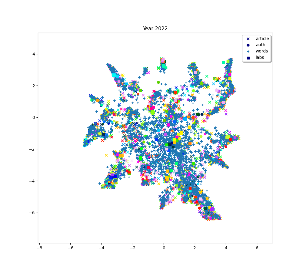
Plot maps
To plot the maps, we will reorganize the data.
def update_embeddings_with_entities(embeddings, filtered_scores):
    r_embeddings = []

    for embedding, score in zip(embeddings, filtered_scores):
        score_indices = np.matrix(score.index).T
        embd = np.hstack((embedding, score_indices)).T
        r_embeddings.append(np.asarray(embd))

    return r_embeddings


def decompose_embeddings(embeddings):
    article_embeddings = []
    auth_embeddings = []
    word_embeddings = []
    lab_embeddings = []

    for i, embedding in enumerate(embeddings):
        len_article = len(scores_article[i])
        len_auth = len(filtered_auth_scores[i])
        len_word = len(words_scores[i])

        article_embeddings.append(embeddings[i][:len_article])
        auth_embeddings.append(
            embeddings[i][len_article: len_article + len_auth])
        word_embeddings.append(
            embeddings[i][len_article + len_auth:len_article + len_auth + len_word])
        lab_embeddings.append(
            embeddings[i][len_article + len_auth + len_word:])

    return article_embeddings, auth_embeddings, word_embeddings, lab_embeddings


article_embeddings, auth_embeddings, word_embeddings, lab_embeddings = decompose_embeddings(
    reducer.embeddings_)
We will add values to embeddings, so that we can visualize article title, author name, word or lab name when the entity is hovered on the plot.
article_embeddings_names = update_embeddings_with_entities(
    article_embeddings, scores_article
)

auth_embeddings_names = update_embeddings_with_entities(
    auth_embeddings, filtered_auth_scores
)

word_embeddings_names = update_embeddings_with_entities(
    word_embeddings, words_scores
)

lab_embeddings_names = update_embeddings_with_entities(
    lab_embeddings, filtered_lab_scores
)
We will create a colormap that will map each entity (article, author, word, lab) to same color in every plot.
from matplotlib import cm   # noqa


def create_color_map(max_list):
    cmap = cm.get_cmap('gist_ncar', len(max_list))
    return cmap


cmap_article = create_color_map(scores_article[-1])
cmap_auth = create_color_map(filtered_auth_scores[-1])
cmap_word = create_color_map(words_scores[-1])
cmap_lab = create_color_map(filtered_lab_scores[-1])
/builds/2mk6rsew/0/hgozukan/cartolabe-data/examples/workflow_aligned_lisn_lsa_kmeans.py:634: MatplotlibDeprecationWarning: The get_cmap function was deprecated in Matplotlib 3.7 and will be removed in 3.11. Use ``matplotlib.colormaps[name]`` or ``matplotlib.colormaps.get_cmap()`` or ``pyplot.get_cmap()`` instead.
  cmap = cm.get_cmap('gist_ncar', len(max_list))
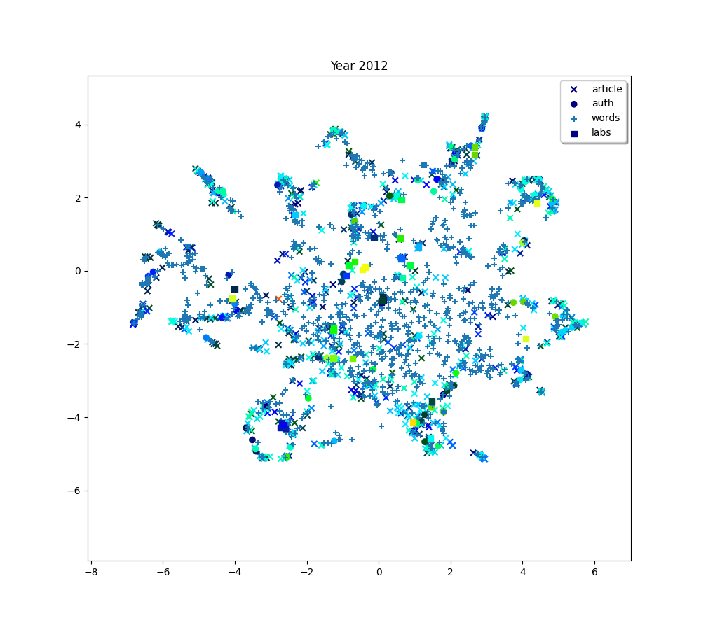
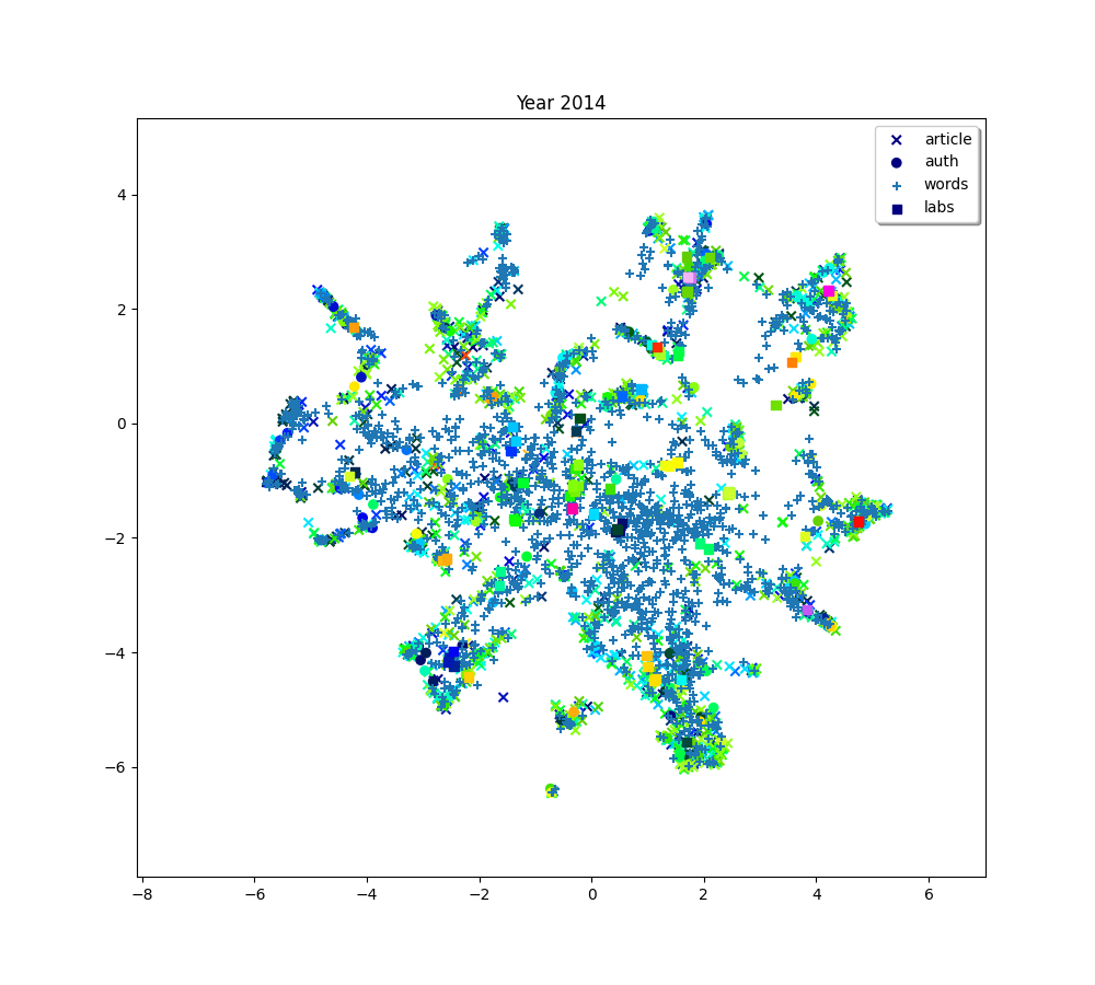
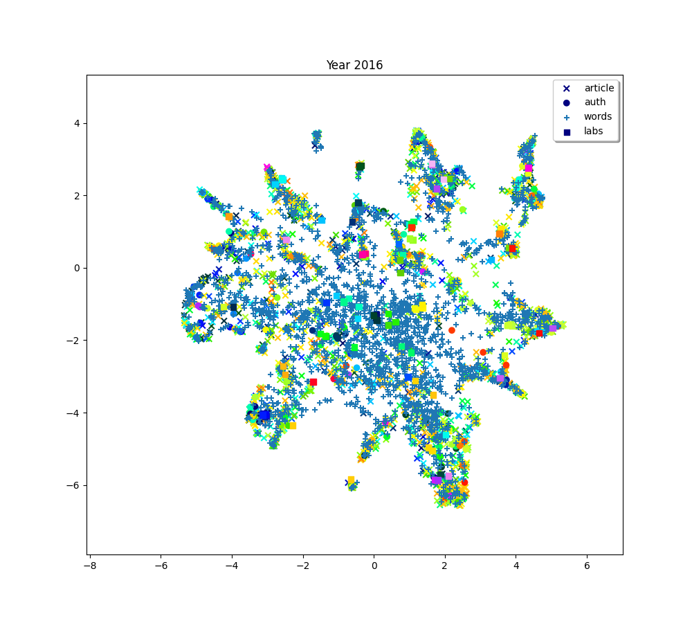
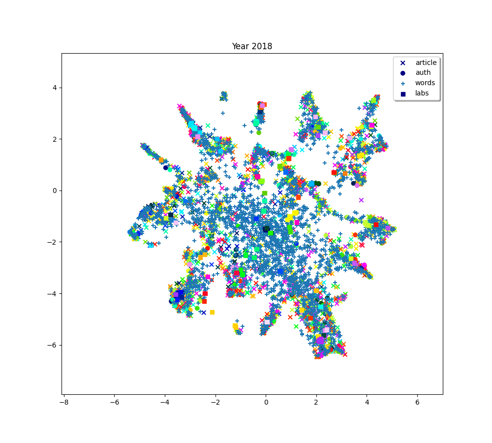
Now we can plot all the maps.
import matplotlib.pyplot as plt  # noqa
import numpy as np   # noqa
import mplcursors    # noqa


plt.close('all')

def axis_bounds(embedding):
    left, right = embedding.T[0].min(), embedding.T[0].max()
    bottom, top = embedding.T[1].min(), embedding.T[1].max()
    adj_h, adj_v = (right - left) * 0.1, (top - bottom) * 0.1

    return [left - adj_h, right + adj_h, bottom - adj_v, top + adj_v]


ax_bound = axis_bounds(np.vstack(reducer.embeddings_))
ax_bound


def plot(title, embedding_article, embedding_auth, embedding_word, embedding_lab,
         colors_article, colors_auth, colors_word, colors_lab,
         c_scores=None, c_umap=None, n_clusters=None):

    colors_article_list = list(colors_article.values())
    colors_auth_list = list(colors_auth.values())
    colors_word_list = list(colors_word.values())
    colors_lab_list = list(colors_lab.values())

    fig, ax = plt.subplots(1, 1, figsize=(10, 9))

    ax.set_title(title)
    ax.axis(ax_bound)

    article = ax.scatter(embedding_article[0], embedding_article[1], c=colors_article_list, cmap=cmap_article,
                         vmin=0, vmax=len(scores_article[-1]), marker='x', label="article")

    auth = ax.scatter(embedding_auth[0], embedding_auth[1], c=colors_auth_list, cmap=cmap_auth,
                      vmin=0, vmax=len(filtered_auth_scores[-1]), label="auth")

    word = ax.scatter(embedding_word[0], embedding_word[1],
                      vmin=0, vmax=len(words_scores[-1]), marker='+', label="word")

    lab = ax.scatter(embedding_lab[0], embedding_lab[1], c=colors_lab_list, cmap=cmap_lab,
                     vmin=0, vmax=len(filtered_lab_scores[-1]), marker='s', label="lab")

    # from https://matplotlib.org/stable/gallery/event_handling/legend_picking.html
    leg = ax.legend((article, auth, word, lab), ("article",
                                                 "auth", "words", "labs"), fancybox=True, shadow=True)

    if n_clusters is not None:
        for i in range(n_clusters):
            ax.annotate(c_scores.index[i], (c_umap[0, i], c_umap[1, i]))

#    crs_article = mplcursors.cursor(article, hover=True)

#    @crs_article.connect("add")
#    def on_add(sel):
#        sel.annotation.set(text=embedding_article[2][sel.target.index])

    crs_auth = mplcursors.cursor(auth, hover=True)

    @crs_auth.connect("add")
    def on_add(sel):
        sel.annotation.set(text=embedding_auth[2][sel.target.index])

#    crs_word = mplcursors.cursor(word, hover=True)

#    @crs_word.connect("add")
#    def on_add(sel):
#        sel.annotation.set(text=embedding_word[2][sel.target.index])

    crs_lab = mplcursors.cursor(lab, hover=True)

    @crs_lab.connect("add")
    def on_add(sel):
        sel.annotation.set(text=embedding_lab[2][sel.target.index])

    plt.show()


for i, (embedding_article, embedding_auth, embedding_word, embedding_lab,
        color_article, color_auth, color_word, color_lab) in enumerate(zip(
    article_embeddings_names, auth_embeddings_names, word_embeddings_names, lab_embeddings_names,
    colors_articles, colors_auth, colors_words, colors_lab)):

    plot(f"Year {2010 + (i * 2) + 2}", embedding_article, embedding_auth, embedding_word, embedding_lab,
         color_article, color_auth, color_word, color_lab)

/usr/local/lib/python3.9/site-packages/mplcursors/_pick_info.py:55: UserWarning: No data for colormapping provided via 'c'. Parameters 'vmin', 'vmax' will be ignored
  paths = scatter.__wrapped__(*args, **kwargs)
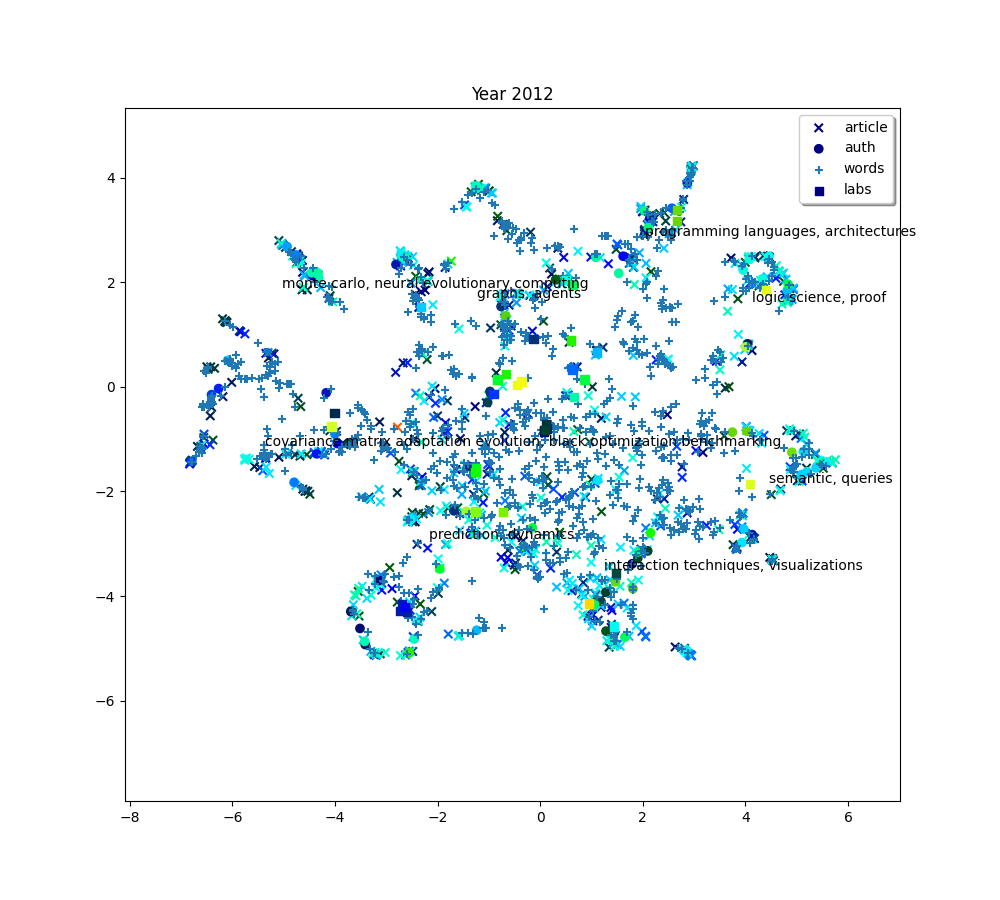
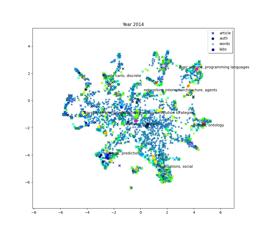
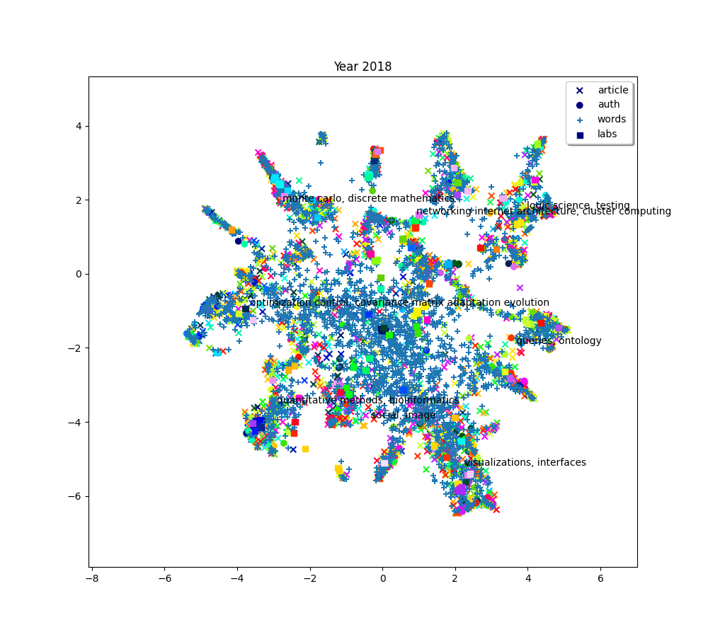
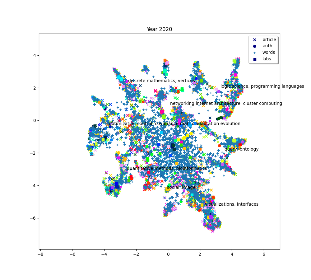
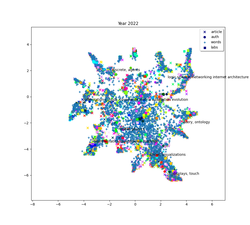
Clustering
In order to identify clusters, we use the KMeans clustering technique on the articles. We’ll also try to label these clusters by selecting the most frequent words that appear in each cluster’s articles.
from cartodata.clustering import create_kmeans_clusters  # noqa
n_clusters = 8


def find_clusters(n_clusters, article_embeddings, word_embeddings,
                  words_matrices, words_scores, matrices):

    c_scores_all = []
    c_umap_all = []

    for i in range(6):
        cluster_labels = []
        c_lda, c_umap, c_scores, c_knn, _, _, _ = create_kmeans_clusters(n_clusters,  # number of clusters to create
                                                                # 2D matrix of articles
                                                                article_embeddings[i].T,
                                                                # the 2D matrix of words
                                                                word_embeddings[i].T,
                                                                # the articles to words matrix
                                                                words_matrices[i],
                                                                # word scores
                                                                words_scores[i],
                                                                # a list of initial cluster labels
                                                                cluster_labels,
                                                                # space matrix of words
                                                                matrices[i][2])
        c_scores_all.append(c_scores)
        c_umap_all.append(c_umap)

    return c_scores_all, c_umap_all


c_scores_all, c_umap_all = find_clusters(n_clusters, article_embeddings, word_embeddings,
                                         words_matrices, words_scores, lsa_matrices)
Let’s plot with the clusters.
for i, (embedding_article, embedding_auth, embedding_word, embedding_lab,
        color_article, color_auth, color_word, color_lab, c_scores, c_umap) in enumerate(zip(
    article_embeddings_names, auth_embeddings_names, word_embeddings_names, lab_embeddings_names,
    colors_articles, colors_auth, colors_words, colors_lab, c_scores_all, c_umap_all)):

    plot(f"Year {2010+ (i*2) + 2}", embedding_article, embedding_auth, embedding_word, embedding_lab,
         color_article, color_auth, color_word, color_lab, c_scores, c_umap, n_clusters)

/usr/local/lib/python3.9/site-packages/mplcursors/_pick_info.py:55: UserWarning: No data for colormapping provided via 'c'. Parameters 'vmin', 'vmax' will be ignored
  paths = scatter.__wrapped__(*args, **kwargs)
The 8 clusters that we created give us a general idea of what the big clusters of data contain. But we’ll probably want a finer level of detail if we start to zoom in and focus on smaller areas. So we’ll also create a second bigger group of clusters. To do this, simply increase the number of clusters we want.
n_clusters = 32

mc_scores_all, mc_umap_all = find_clusters(
    n_clusters, article_embeddings, word_embeddings, words_matrices, words_scores, lsa_matrices
)
Nearest neighbors
One more thing which could be useful to appreciate the quality of our data would be to get each point’s nearest neighbors. If our data processing is done correctly, we expect the related articles, labs, words and authors to be located close to each other.
Finding nearest neighbors is a common task with various algorithms aiming to solve it. The get_neighbors method uses one of these algorithms to find the nearest points of each type. It takes an optional weight parameter to tweak the distance calculation to select points that have a higher score but are maybe a bit farther instead of just selecting the closest neighbors.
Because we want to find the neighbors of each type (articles, authors, words, labs) for all of the entities, we call the get_neighbors method in a loop and store its results in an array.
from cartodata.neighbors import get_neighbors  # noqa


def find_neighbors(articles_scores, authors_scores, words_scores,
                   labs_scores, matrices):

    weights = [0, 0.5, 0.5, 0]

    all_neighbors = []
    all_scores = []

    for i in range(6):
        scores = [articles_scores[i], authors_scores[i],
                  words_scores[i], labs_scores[i]]
        neighbors = []

        matrix = matrices[i]
        for idx in range(len(matrix)):
            neighbors.append(get_neighbors(matrix[idx],
                                           scores[idx],
                                           matrix,
                                           weights[idx])
                                 )
        all_neighbors.append(neighbors)
        all_scores.append(scores)

    return all_neighbors, all_scores


all_neighbors, all_scores = find_neighbors(scores_article, filtered_auth_scores,
                                           words_scores, filtered_lab_scores, lsa_matrices)
Exporting
We now have sufficient data to create a meaningfull visualization.
from cartodata.operations import export_to_json  # noqa

natures = ['articles',
           'authors',
           'words',
           'labs',
           'hl_clusters',
           'ml_clusters']


def export(from_year, struct, article_embeddings, authors_embeddings, word_embeddings, lab_embeddings,
           c_umap, mc_umap, c_scores, mc_scores, all_neighbors, all_scores):


    for i in range(6):
        export_file = f"../datas/{struct}_workflow_lsa_aligned_{from_year}_{from_year + (2 + 2 * i)}.json"

        # add the clusters to list of 2d matrices and scores
        umap_matrices = [article_embeddings[i].T,
                         authors_embeddings[i].T,
                         word_embeddings[i].T,
                         lab_embeddings[i].T,
                         c_umap[i],
                         mc_umap[i]]

        all_scores[i].extend([c_scores[i], mc_scores[i]])


        # create a json export file with all the infos
        export_to_json(natures,
                       umap_matrices,
                       all_scores[i],
                       export_file,
                       neighbors_natures=natures[:4],
                       neighbors=all_neighbors[i])


export(2010, "lisn", article_embeddings, auth_embeddings, word_embeddings, lab_embeddings,
           c_umap_all, mc_umap_all, c_scores_all, mc_scores_all, all_neighbors, all_scores)
This creates the files:
lisn_workflow_aligned_lsa_2010_2012.json
lisn_workflow_aligned_lsa_2010_2014.json
lisn_workflow_aligned_lsa_2010_2016.json
lisn_workflow_aligned_lsa_2010_2018.json
lisn_workflow_aligned_lsa_2010_2020.json
lisn_workflow_aligned_lsa_2010_2022.json
each of which contains a list of points ready to be imported into Cartolabe. Have a look at it to check that it contains everything.
import json  # noqa

export_file = "../datas/lisn_workflow_lsa_aligned_2010_2022.json"

with open(export_file, 'r') as f:
    data = json.load(f)

data[1]
{'position': [-4.62356424331665, 1.2929304838180542], 'score': 1.0, 'rank': 1, 'nature': 'articles', 'label': 'Bandit-Based Genetic Programming with Application to Reinforcement Learning', 'neighbors': {'articles': [1, 216, 48, 443, 952, 1596, 2623, 78, 323, 1552], 'authors': [3044, 3034, 3026, 3046, 3152, 2987, 3086, 3088, 3043, 3028], 'words': [3767, 5394, 5395, 5396, 3768, 6285, 6340, 6339, 6303, 6230], 'labs': [7032, 6944, 7011, 6989, 7018, 7017, 6985, 7016, 7030, 7076]}}
Total running time of the script: (15 minutes 59.159 seconds)