Note
Go to the end to download the full example code.
Extracting and processing LISN data for Cartolabe ( Doc2vec projection)
In this example we will:
extract entities (authors, articles, labs, words) from a collection of scientific articles
project those entities in 2 dimensions
cluster them
find their nearest neighbors.
Download data
We will first download the CSV file that contains all articles from HAL (https://hal.archives-ouvertes.fr/) published by authors from LISN (Laboratoire Interdisciplinaire des Sciences du Numérique) between 2000-2022.
from download import download

csv_url = "https://zenodo.org/record/7323538/files/lisn_2000_2022.csv"

download(csv_url, "../datas/lisn_2000_2022.csv", kind='file',
                         progressbar=True, replace=False)
Replace is False and data exists, so doing nothing. Use replace=True to re-download the data.

'../datas/lisn_2000_2022.csv'
Load data to dataframe
import pandas as pd  # noqa

df = pd.read_csv('../datas/lisn_2000_2022.csv', index_col=0)

df.head()
The dataframe that we just read consists of 4262 articles as rows.
print(df.shape[0])
4262
And their authors, abstract, keywords, title, research labs and domain as columns.
print(*df.columns, sep="\n")
structId_i
authFullName_s
en_abstract_s
en_keyword_s
en_title_s
structAcronym_s
producedDateY_i
producedDateM_i
halId_s
docid
en_domainAllCodeLabel_fs
Creating correspondance matrices for each entity type
From this table of articles, we want to extract matrices that will map the correspondance between these articles and the entities we want to use.
Labs
Similarly, we can create matrices for the labs by simply passing the structAcronym_s column to the function.
labs_mat, labs_scores = load_comma_separated_column(df,
                                                    'structAcronym_s',
                                                    filter_acronyms=True
                                                    )
labs_scores.head()
LRI      4789
UP11     6271
CNRS    10217
LISN     5203
LMS         1
dtype: int64
Checking the number of columns of the sparse matrix labs_mat, we see that there are 1818 distict labs.
labs_mat.shape[1]
1818
Filtering low score entities
A lot of the authors and labs that we just extracted from the dataframe have a very low score, which means they’re only linked to one or two articles. To improve the quality of our data, we’ll filter the authors and labs by removing those that appear less than 4 times.
To do this, we’ll use the filter_min_score function.
from cartodata.operations import filter_min_score  # noqa

authors_before = len(authors_scores)
labs_before = len(labs_scores)

authors_mat, authors_scores = filter_min_score(authors_mat,
                                               authors_scores,
                                               4)
labs_mat, labs_scores = filter_min_score(labs_mat,
                                         labs_scores,
                                         4)

print(f"Removed {authors_before - len(authors_scores)} authors with less "
      f"than 4 articles from a total of {authors_before} authors.")
print(f"Working with {len(authors_scores)} authors.\n")

print(f"Removed {labs_before - len(labs_scores)} labs with less than "
      f"4 articles from a total of {labs_before}.")
print(f"Working with {len(labs_scores)} labs.")
Removed 6654 authors with less than 4 articles from a total of 7348 authors.
Working with 694 authors.

Removed 1255 labs with less than 4 articles from a total of 1818.
Working with 563 labs.
Words
For the words, it’s a bit trickier because we want to extract n-grams (groups of n terms) instead of just comma separated values. We’ll call the load_text_column which uses scikit-learn’s CountVectorizer to create a vocabulary and map the tokens.
from cartodata.loading import load_text_column  # noqa
from sklearn.feature_extraction import text as sktxt  # noqa

with open('../datas/stopwords.txt', 'r') as stop_file:
    stopwords = sktxt.ENGLISH_STOP_WORDS.union(
        set(stop_file.read().splitlines()))

df['text'] = df['en_abstract_s'] + ' ' \
    + df['en_keyword_s'].astype(str) + ' ' \
    + df['en_title_s'].astype(str) + ' ' \
    + df['en_domainAllCodeLabel_fs'].astype(str)

words_mat, words_scores = load_text_column(df['text'],
                                           4,
                                           10,
                                           0.05,
                                           stopwords=stopwords)
Here words_scores contains a list of all the n-grams extracted from the documents with their score,
words_scores.head()
abilities     21
ability      164
absence       53
absolute      19
abstract     174
dtype: int64
and the words_mat matrix counts the occurences of each of the 3457 n-grams for all the articles.
words_mat.shape
(4262, 4682)
To get a better representation of the importance of each term, we’ll also apply a TF-IDF (term-frequency times inverse document-frequency) normalization on the matrix.
The normalize_tfidf simply calls scikit-learn’s TfidfTransformer class.
from cartodata.operations import normalize_tfidf  # noqa

words_mat = normalize_tfidf(words_mat)
Articles
Finally, we need to create a matrix that simply maps each article to itself.
from cartodata.loading import load_identity_column  # noqa

articles_mat, articles_scores = load_identity_column(df, 'en_title_s')
articles_scores.head()
Termination and Confluence of Higher-Order Rewrite Systems                                    1.0
Efficient Self-stabilization                                                                  1.0
Resource-bounded relational reasoning: induction and deduction through stochastic matching    1.0
Reasoning about generalized intervals : Horn representability and tractability                1.0
Proof Nets and Explicit Substitutions                                                         1.0
dtype: float64
Dimension reduction
One way to see the matrices that we created is as coordinates in the space of all articles. What we want to do is to reduce the dimension of this space to make it easier to work with and see.
Doc2vec projection
This example uses the Doc2vec technique to identify keywords in our data and thus reduce the number of rows in our matrices. The doc2vec_projection method takes at least four arguments:
the number of dimensions you want to keep
the matrix identifier of documents/words frequency
a list of matrices to project
the list of text to index (it is possible to add doc2vec parameters with the same syntax of the gensim doc2vec function).
It returns a list of matrices projected in the latent space.
We also apply an l2 normalization to each feature of the projected matrices.
from cartodata.projection import doc2vec_projection  # noqa
from cartodata.operations import normalize_l2  # noqa

doc2vec_matrices = doc2vec_projection(50,
                                  2,
                                  [articles_mat, authors_mat, words_mat,
                                   labs_mat],
                                  df['text'])
doc2vec_matrices = list(map(normalize_l2, doc2vec_matrices))
We’ve reduced the number of rows in each of articles_mat, authors_mat, words_mat and labs_mat to just 50.
print(f"articles_mat: {doc2vec_matrices[0].shape}")
print(f"authors_mat: {doc2vec_matrices[1].shape}")
print(f"words_mat: {doc2vec_matrices[2].shape}")
print(f"labs_mat: {doc2vec_matrices[3].shape}")
articles_mat: (50, 4262)
authors_mat: (50, 694)
words_mat: (50, 4682)
labs_mat: (50, 563)
This makes it easier to work with them for clustering or nearest neighbors tasks, but we also want to project them on a 2D space to be able to map them.
UMAP projection
The UMAP (Uniform Manifold Approximation and Projection) is a dimension reduction technique that can be used for visualisation similarly to t-SNE.
We use this algorithm to project our matrices in 2 dimensions.
from cartodata.projection import umap_projection  # noqa

umap_matrices = umap_projection(doc2vec_matrices)
Now that we have 2D coordinates for our points, we can try to plot them to get a feel of the data’s shape.
import matplotlib.pyplot as plt  # noqa
import numpy as np  # noqa
import seaborn as sns  # noqa
# %matplotlib inline

sns.set(style='white', rc={'figure.figsize': (12, 8)})

labels = ('article', "auth", "words", "labs")
colors = ['g', 'r', 'b', 'y']
markers = ['o', 's', '+', 'x']

def plot(matrices):
    plt.close('all')
    fig, ax = plt.subplots()

    axes = []

    for i, m in enumerate(matrices):
        axes.append(ax.scatter(m[0, :], m[1, :],
                               color=colors[i], marker=markers[i],
                               label = labels[i]))


    leg = ax.legend((axes[0], axes[1], axes[2], axes[3]),
                    labels,
                    fancybox=True, shadow=True)

    return fig, ax

fig, ax = plot(umap_matrices)
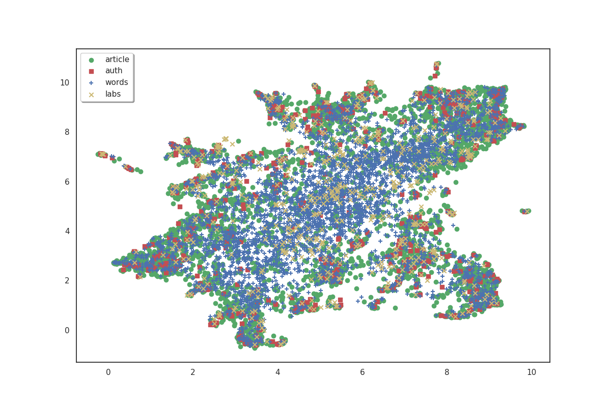
On the plot above, articles are shown in green, authors in red, words in blue and labs in yellow. Because we don’t have labels for the points, it doesn’t make much sense as is. But we can see that the data shows some clusters which we could try to identify.
Clustering
In order to identify clusters, we use the KMeans clustering technique on the articles. We’ll also try to label these clusters by selecting the most frequent words that appear in each cluster’s articles.
from cartodata.clustering import create_kmeans_clusters  # noqa

cluster_labels = []
c_lda, c_umap, c_scores, c_knn, _, _, _ = create_kmeans_clusters(8,  # number of clusters to create
                                                        # 2D matrix of articles
                                                        umap_matrices[0],
                                                        # the 2D matrix of words
                                                        umap_matrices[2],
                                                        # the articles to words matrix
                                                        words_mat,
                                                        # word scores
                                                        words_scores,
                                                        # a list of initial cluster labels
                                                        cluster_labels,
                                                        # LDA space matrix of words
                                                        doc2vec_matrices[2])

c_scores

""
fig, ax = plot(umap_matrices)

for i in range(8):
    ax.annotate(c_scores.index[i], (c_umap[0, i], c_umap[1, i]),
                color='red')
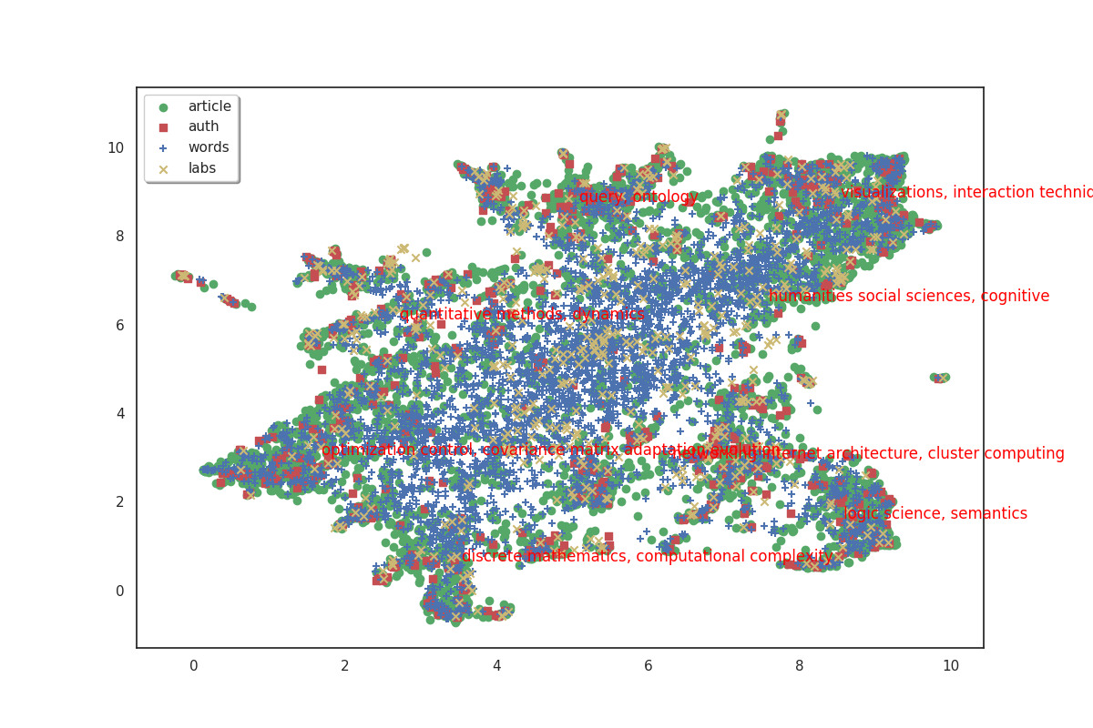
The 8 clusters that we created give us a general idea of what the big clusters of data contain. But we’ll probably want a finer level of detail if we start to zoom in and focus on smaller areas. So we’ll also create a second bigger group of clusters. To do this, simply increase the number of clusters we want.
mc_lsa, mc_umap, mc_scores, mc_knn, _, _, _ = create_kmeans_clusters(32,
                                                            umap_matrices[0],
                                                            umap_matrices[2],
                                                            words_mat,
                                                            words_scores,
                                                            cluster_labels,
                                                            doc2vec_matrices[2])
mc_scores
molecular, metabolism                                 94
systems biology, regulatory networks                  88
human interaction, interfaces                        198
discrete, combinatorics                              176
specification, programming languages                 161
scientific workflows, information theoretic           99
inference, evolutionary robotics                     169
linear systems, discrete event systems               113
stochastic, integer linear programming               131
ontologies, information retrieval                    201
modeling simulation, services                        111
monte carlo, parameter                               175
social sciences, community                           175
neural networks, adaptation strategies               100
networking internet, consumption                     170
architectures, storage                               193
abstract model, simulators                            63
stabilizing, protocols                               105
display, touch                                       172
graph searching, maximum degree                       25
queries, resource description framework              144
large hadron collider, machine learning challenge     20
participants, argue                                  135
challenge, machine translation                       100
secondary structure, structural                      102
french, multilingual                                 119
numerical simulations, fluid                         111
vertices, minimum                                    129
verification, proof assistant                        193
convolutional neural networks, trained                91
evolution strategies, testbed                        214
representations, exploring                           185
dtype: int64
Nearest neighbors
One more thing which could be useful to appreciate the quality of our data would be to get each point’s nearest neighbors. If our data processing is done correctly, we expect the related articles, labs, words and authors to be located close to each other.
Finding nearest neighbors is a common task with various algorithms aiming to solve it. The get_neighbors method uses one of these algorithms to find the nearest points of each type. It takes an optional weight parameter to tweak the distance calculation to select points that have a higher score but are maybe a bit farther instead of just selecting the closest neighbors.
Because we want to find the neighbors of each type (articles, authors, words, labs) for all of the entities, we call the get_neighbors method in a loop and store its results in an array.
from cartodata.neighbors import get_neighbors  # noqa

scores = [articles_scores, authors_scores, words_scores, labs_scores]
weights = [0, 0.5, 0.5, 0]
all_neighbors = []

for idx in range(len(doc2vec_matrices)):
    all_neighbors.append(get_neighbors(doc2vec_matrices[idx],
                                       scores[idx],
                                       doc2vec_matrices,
                                       weights[idx]))
Exporting
We now have sufficient data to create a meaningfull visualization.
from cartodata.operations import export_to_json  # noqa

natures = ['articles',
           'authors',
           'words',
           'labs',
           'hl_clusters',
           'ml_clusters'
           ]
export_file = '../datas/lisn_workflow_doc2vec.json'

# add the clusters to list of 2d matrices and scores
matrices = list(umap_matrices)
matrices.extend([c_umap, mc_umap])
scores.extend([c_scores, mc_scores])

# create a json export file with all the infos
export_to_json(natures,
               matrices,
               scores,
               export_file,
               neighbors_natures=natures[:4],
               neighbors=all_neighbors)
This creates the lisn_workflow_doc2vec.json file which contains a list of points ready to be imported into Cartolabe. Have a look at it to check that it contains everything.
import json  # noqa

with open(export_file, 'r') as f:
    data = json.load(f)

data[1]['position']
[4.724753379821777, 0.9927496314048767]
Total running time of the script: (1 minutes 12.205 seconds)