Note
Go to the end to download the full example code.
Extracting and processing VisPubData data for Cartolabe
In this example we will:
extract entities (authors, articles, labs, words) from a collection of scientific articles
project those entities in 2 dimensions
cluster them
find their nearest neighbors.
Download data
We will first download the CSV file that contains all the scientific articles published to the VIS conference between 1990 and 2019. The CSV is maintained on the VisPubData web site.
from download import download

csv_url = "https://zenodo.org/record/7569091/files/vispubdata_1990_2019.csv"

download(csv_url, "../datas/vispubdata_1990_2019.csv", kind='file',
                         progressbar=True, replace=False)

""
import pandas as pd   # noqa

df = pd.read_csv('../datas/vispubdata_1990_2019.csv')
df.dropna(subset=['Abstract'], inplace=True)

df.head()
Downloading data from https://zenodo.org/records/7569091/files/vispubdata_1990_2019.csv (4.7 MB)


file_sizes:   0%|                                   | 0.00/4.97M [00:00<?, ?B/s]
file_sizes:  73%|██████████████████▉       | 3.63M/4.97M [00:00<00:00, 36.1MB/s]
file_sizes: 100%|██████████████████████████| 4.97M/4.97M [00:00<00:00, 43.9MB/s]
Successfully downloaded file to ../datas/vispubdata_1990_2019.csv
The dataset contains 3028 articles.
print(df.shape[0])
3028
Let’s list the columns:
print(*df.columns, sep="\n")
Conference
Year
Title
DOI
Link
FirstPage
LastPage
PaperType
Abstract
AuthorNames-Deduped
AuthorNames
AuthorAffiliation
InternalReferences
AuthorKeywords
AminerCitationCount_02-2019
XPloreCitationCount_02-2019
PubsCited
Award
Creating correspondance matrices for each entity type
From this table of articles, we want to extract matrices that will map the correspondance between these articles and the entities we want to use.
Filtering low score entities
A lot of the authors and labs that we just extracted from the dataframe have a very low score, which means they’re only linked to one or two articles. To improve the quality of our data, we’ll filter the authors and labs by removing those that appear less than 2 times.
To do this, we’ll use the filter_min_score function.
from cartodata.operations import filter_min_score   # noqa

authors_before = len(authors_scores)
authors_mat, authors_scores = filter_min_score(authors_mat, authors_scores, 2)

print(f"Removed {authors_before - len(authors_scores)} authors with less than 2 "
      f"articles from a total of {authors_before} authors.")
print(f"Working with {len(authors_scores)} authors.\n")
Removed 4569 authors with less than 2 articles from a total of 5405 authors.
Working with 836 authors.
Words
For the words, it’s a bit trickier because we want to extract n-grams (groups of n terms) instead of just comma separated values. We’ll call the load_text_column which uses scikit-learn’s CountVectorizer to create a vocabulary and map the tokens.
from cartodata.loading import load_text_column   # noqa
from sklearn.feature_extraction import text as sktxt   # noqa

with open('../datas/stopwords.txt', 'r') as stop_file:
    stopwords = sktxt.ENGLISH_STOP_WORDS.union(
        set(stop_file.read().splitlines()))

df['text'] = df['Abstract'] + ' ' \
    + df['AuthorKeywords'].astype(str) + ' ' \
    + df['Title']  # maybe add more

words_mat, words_scores = load_text_column(df['text'],
                                           4,
                                           10,
                                           0.05,
                                           stopwords=stopwords)
Here words_scores contains a list of all the n-grams extracted from the documents with their score,
words_scores.head()
abilities       31
ability        133
absolute        12
abstract        81
abstraction     73
dtype: int64
and the words_mat matrix counts the occurences of each of the 3387 n-grams for all the articles.
words_mat.shape
(3028, 3387)
To get a better representation of the importance of each term, we’ll also apply a TF-IDF (term-frequency times inverse document-frequency) normalization on the matrix.
The normalize_tfidf simply calls scikit-learn’s TfidfTransformer class.
from cartodata.operations import normalize_tfidf   # noqa

words_mat = normalize_tfidf(words_mat)
Articles
Finally, we need to create a matrix that simply maps each article to itself.
df['XPloreCitationCount_02-2019']

""
from cartodata.loading import load_identity_column   # noqa
import scipy.sparse as scs   # noqa

# articles_mat, articles_scores = load_identity_column(df, 'Title')
titles = df['Title']
articles_mat = scs.identity(len(titles))
articles_scores = pd.Series(df['XPloreCitationCount_02-2019'].values + 1,
                            index=titles)

articles_scores.head()
Title
Surface representations of two- and three-dimensional fluid flow topology                24.0
FAST: a multi-processed environment for visualization of computational fluid dynamics    30.0
The VIS-5D system for easy interactive visualization                                     25.0
A procedural interface for volume rendering                                               4.0
Techniques for the interactive visualization of volumetric data                           8.0
dtype: float64
Dimension reduction
One way to see the matrices that we created is as coordinates in the space of all articles. What we want to do is to reduce the dimension of this space to make it easier to work with and see.
LSA projection
We’ll start by using the LSA (Latent Semantic Analysis) technique to identify keywords in our data and thus reduce the number of rows in our matrices. The lsa_projection method takes three arguments:
the number of dimensions you want to keep
the matrix of documents/words frequency
a list of matrices to project
It returns a list of the same length containing the matrices projected in the latent space.
We also apply an l2 normalization to each feature of the projected matrices.
from cartodata.projection import lsa_projection   # noqa
from cartodata.operations import normalize_l2   # noqa

lsa_matrices = lsa_projection(80,
                              words_mat,
                              [articles_mat, authors_mat, words_mat])
lsa_matrices = list(map(normalize_l2, lsa_matrices))
We’ve reduced the number of rows in each of articles_mat, authors_mat, words_mat and labs_mat to just 80.
print(f"articles_mat: {lsa_matrices[0].shape}")
print(f"authors_mat: {lsa_matrices[1].shape}")
print(f"words_mat: {lsa_matrices[2].shape}")
articles_mat: (80, 3028)
authors_mat: (80, 836)
words_mat: (80, 3387)
This makes it easier to work with them for clustering or nearest neighbors tasks, but we also want to project them on a 2D space to be able to map them.
UMAP projection
The UMAP (Uniform Manifold Approximation and Projection) is a dimension reduction technique that can be used for visualisation similarly to t-SNE.
We use this algorithm to project our matrices in 2 dimensions.
from cartodata.projection import umap_projection   # noqa

umap_matrices = umap_projection(lsa_matrices)
Now that we have 2D coordinates for our points, we can try to plot them to get a feel of the data’s shape.
import matplotlib.pyplot as plt  # noqa
import numpy as np  # noqa
import seaborn as sns  # noqa
# %matplotlib inline

sns.set(style='white', rc={'figure.figsize': (12, 8)})

labels = ('article', "auth", "words")
colors = ['g', 'r', 'b']
markers = ['x', 's', '+']

def plot(matrices):
    plt.close('all')
    fig, ax = plt.subplots()

    axes = []

    for i, m in enumerate(matrices):
        axes.append(ax.scatter(m[0, :], m[1, :],
                               color=colors[i], marker=markers[i],
                               label = labels[i]))


    leg = ax.legend((axes[0], axes[1], axes[2]),
                    labels,
                    fancybox=True, shadow=True)

    return fig, ax

fig, ax = plot(umap_matrices)
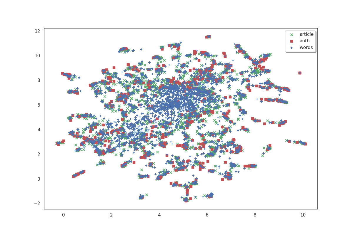
On the plot above, articles are shown in green, authors in red and words in blue. Because we don’t have labels for the points, it doesn’t make much sense as is. But we can see that the data shows some clusters which we could try to identify.
Clustering
In order to identify clusters, we use the KMeans clustering technique on the articles. We’ll also try to label these clusters by selecting the most frequent words that appear in each cluster’s articles.
from cartodata.clustering import create_kmeans_clusters  # noqa

cluster_labels = []
c_lda, c_umap, c_scores, c_knn, _, _, _ = create_kmeans_clusters(8,  # number of clusters to create
                                                        # 2D matrix of articles
                                                        umap_matrices[0],
                                                        # the 2D matrix of words
                                                        umap_matrices[2],
                                                        # the articles to words matrix
                                                        words_mat,
                                                        # word scores
                                                        words_scores,
                                                        # a list of initial cluster labels
                                                        cluster_labels,
                                                        # LDA space matrix of words
                                                        lsa_matrices[2])

c_scores

""
fig, ax = plot(umap_matrices)

for i in range(8):
    ax.annotate(c_scores.index[i], (c_umap[0, i], c_umap[1, i]),
                color='red')

The 8 clusters that we created give us a general idea of what the big clusters of data contain. But we’ll probably want a finer level of detail if we start to zoom in and focus on smaller areas. So we’ll also create a second bigger group of clusters. To do this, simply increase the number of clusters we want.
mc_lsa, mc_umap, mc_scores, mc_knn, _, _, _ = create_kmeans_clusters(32,
                                                            umap_matrices[0],
                                                            umap_matrices[2],
                                                            words_mat,
                                                            words_scores,
                                                            cluster_labels,
                                                            lsa_matrices[2])

mc_scores
graph visualization, diagrams            129
vector fields, critical points           114
events, detection                         96
interpolation, surface reconstruction    108
visualization design, design process      99
visualization systems, program           121
virtual reality, parameter space         101
tracking, sequence                        48
networks, topic                           97
ensemble, weather                         31
uncertainty, cluster                     103
diffusion tensor, tensor field            98
imaging, segmentation                    142
video, multi projector                    50
object, distributed                      128
particle, motion                          83
machine learning, classification          65
analytic, collaborative                  134
coordinates, variables                   128
isosurface                                52
illumination, volume visualization       125
multiresolution, grids                   106
focus context, trees                      97
participants, perceptual                 126
traffic, spatio                           75
finite element                            32
computational fluid dynamics, vortex      86
compression, simplification               94
decision making, visualisation            99
document, contest                         65
transfer function, contour                74
queries, attributes                      122
dtype: int64
Nearest neighbors
One more thing which could be useful to appreciate the quality of our data would be to get each point’s nearest neighbors. If our data processing is done correctly, we expect the related articles, labs, words and authors to be located close to each other.
Finding nearest neighbors is a common task with various algorithms aiming to solve it. The get_neighbors method uses one of these algorithms to find the nearest points of each type. It takes an optional weight parameter to tweak the distance calculation to select points that have a higher score but are maybe a bit farther instead of just selecting the closest neighbors.
Because we want to find the neighbors of each type (articles, authors, words, labs) for all of the entities, we call the get_neighbors method in a loop and store its results in an array.
from cartodata.neighbors import get_neighbors   # noqa

scores = [articles_scores, authors_scores, words_scores]
weights = [0, 0.5, 0.5, 0]
all_neighbors = []

for idx in range(len(lsa_matrices)):
    all_neighbors.append(get_neighbors(lsa_matrices[idx],
                                       scores[idx],
                                       lsa_matrices,
                                       weights[idx]))
Exporting
We now have sufficient data to create a meaningfull visualization.
We can now export the data. We will first create the exporter.
from cartodata.operations import export_to_json  # noqa

natures = ['articles',
           'authors',
           'words',
           'hl_clusters',
           'ml_clusters'
           ]
export_file = '../datas/vispubdata_lsa.json'

# add the clusters to list of 2d matrices and scores
matrices = list(umap_matrices)
matrices.extend([c_umap, mc_umap])
scores.extend([c_scores, mc_scores])

# Create a json export file with all the infos
export_to_json(natures,
               matrices,
               scores,
               export_file,
               neighbors_natures=natures[:3],
               neighbors=all_neighbors)
This creates the visupubdata_lsa.json file which contains a list of points ready to be imported into Cartolabe. Have a look at it to check that it contains everything.
import json  # noqa

with open(export_file, 'r') as f:
    data = json.load(f)

data[1]['position']
[7.1067399978637695, 1.123482584953308]
Total running time of the script: (0 minutes 38.017 seconds)