Note
Go to the end to download the full example code.
Creating a corpus from Wikipedia
In this example, we’ll describe how to run a text processing workflow on a dump of Wikipedia. We’ll be working with a dump of the Simple English Wikipedia because it is both much smaller than the full English Wikipedia (it has approximately 140000 articles) and the articles have a simpler syntax.
Prepare Simple English Wikipedia Data
Download data
To begin, you must download the latest dump of the Simple English Wikipedia from here (~188M).
from download import download  # noqa

download("https://dumps.wikimedia.org/simplewiki/latest/simplewiki-latest-pages-articles.xml.bz2",
         "../datas/simplewiki-latest-pages-articles.xml.bz2")
Downloading data from https://dumps.wikimedia.org/simplewiki/latest/simplewiki-latest-pages-articles.xml.bz2 (286.7 MB)


file_sizes:   0%|                                    | 0.00/301M [00:00<?, ?B/s]
file_sizes:   2%|▌                          | 6.28M/301M [00:00<00:06, 46.7MB/s]
file_sizes:   6%|█▋                         | 18.9M/301M [00:00<00:03, 85.6MB/s]
file_sizes:  10%|██▋                        | 29.4M/301M [00:00<00:03, 79.2MB/s]
file_sizes:  13%|███▌                       | 39.8M/301M [00:00<00:02, 87.8MB/s]
file_sizes:  17%|████▌                      | 50.3M/301M [00:00<00:02, 84.2MB/s]
file_sizes:  20%|█████▍                     | 60.8M/301M [00:00<00:02, 81.2MB/s]
file_sizes:  23%|██████▏                    | 69.2M/301M [00:00<00:02, 81.2MB/s]
file_sizes:  26%|██████▉                    | 77.6M/301M [00:00<00:02, 76.4MB/s]
file_sizes:  30%|████████                   | 90.2M/301M [00:01<00:02, 87.0MB/s]
file_sizes:  33%|█████████▎                  | 101M/301M [00:01<00:02, 87.7MB/s]
file_sizes:  37%|██████████▎                 | 111M/301M [00:01<00:02, 83.2MB/s]
file_sizes:  40%|███████████▎                | 122M/301M [00:01<00:02, 83.6MB/s]
file_sizes:  44%|████████████▎               | 132M/301M [00:01<00:02, 78.2MB/s]
file_sizes:  48%|█████████████▍              | 145M/301M [00:01<00:01, 86.1MB/s]
file_sizes:  52%|██████████████▍             | 155M/301M [00:01<00:01, 79.4MB/s]
file_sizes:  56%|███████████████▌            | 168M/301M [00:02<00:01, 87.3MB/s]
file_sizes:  59%|████████████████▌           | 178M/301M [00:02<00:01, 87.1MB/s]
file_sizes:  63%|█████████████████▌          | 189M/301M [00:02<00:01, 82.4MB/s]
file_sizes:  66%|██████████████████▌         | 199M/301M [00:02<00:01, 86.3MB/s]
file_sizes:  70%|███████████████████▌        | 210M/301M [00:02<00:01, 78.0MB/s]
file_sizes:  74%|████████████████████▋       | 222M/301M [00:02<00:00, 89.0MB/s]
file_sizes:  77%|█████████████████████▋      | 233M/301M [00:02<00:00, 87.9MB/s]
file_sizes:  81%|██████████████████████▋     | 243M/301M [00:02<00:00, 84.2MB/s]
file_sizes:  84%|███████████████████████▋    | 254M/301M [00:03<00:00, 85.1MB/s]
file_sizes:  88%|████████████████████████▌   | 264M/301M [00:03<00:00, 82.2MB/s]
file_sizes:  91%|█████████████████████████▌  | 275M/301M [00:03<00:00, 87.3MB/s]
file_sizes:  95%|██████████████████████████▌ | 285M/301M [00:03<00:00, 87.7MB/s]
file_sizes:  98%|███████████████████████████▌| 296M/301M [00:03<00:00, 82.0MB/s]
file_sizes: 100%|████████████████████████████| 301M/301M [00:03<00:00, 83.8MB/s]
Successfully downloaded file to ../datas/simplewiki-latest-pages-articles.xml.bz2

'../datas/simplewiki-latest-pages-articles.xml.bz2'
Extract the text from Wikipedia template files
The file we just downloaded is a single dump of all the articles in the simple wikipedia, with templates and markup tags. We want to extract plain text from that, discarding any other information or annotation present in Wikipedia pages, such as images, tables, references and lists.
To do this, we’ll use the WikiExtractor Python package.
import wikiextractor.WikiExtractor as w   # noqa

w.expand_templates = 0
w.Extractor.keepLinks = False
w.Extractor.to_json = True

w.process_dump(input_file="../datas/simplewiki-latest-pages-articles.xml.bz2",
               template_file=None,
               out_file="../datas/simple_wikipedia",
               file_size=(500 * 1024 * 1024),
               file_compress=False,
               process_count=2,
               html_safe=False)
This create datas/simple_wikipedia/AA/wiki_00 json file.
We can now read that file and start working on it.
import pandas as pd   # noqa
import json   # noqa

with open('../datas/simple_wikipedia/AA/wiki_00', 'r') as f:
    docs = f.readlines()

data = list(map(lambda x: json.loads(x), docs))
df = pd.DataFrame(data)
df['text'] = df['text'].str.replace('\\n', ' ', regex=True)

df.head()
Creating correspondance matrices for each entity type
The dataframe that we just read consists of articles as rows and their id, revid, url, title and text as columns.
From this table of articles, we want to extract two matrices representing the articles and their words.
from cartodata.loading import load_text_column   # noqa
from sklearn.feature_extraction import text as sktxt   # noqa

with open('../datas/stopwords.txt', 'r') as stop_file:
    stopwords = sktxt.ENGLISH_STOP_WORDS.union(
        set(stop_file.read().splitlines()))

words_mat, words_scores = load_text_column(df['text'],
                                           4,
                                           10,
                                           0.05,
                                           stopwords=stopwords)
Here words_scores contains a list of all the n-grams extracted from the documents with their score,
words_scores.head()
000th                 30
10000                 43
1000th                23
100th                192
100th anniversary     51
dtype: int64
and the words_mat matrix counts the occurences of each of the 3457 n-grams for all the articles.
words_mat.shape
(357729, 124472)
To get a better representation of the importance of each term, we’ll also apply a TF-IDF (term-frequency times inverse document-frequency) normalization on the matrix.
The normalize_tfidf simply calls scikit-learn’s TfidfTransformer class.
from cartodata.operations import normalize_tfidf  # noqa

words_mat = normalize_tfidf(words_mat)
Articles
Finally, we need to create a matrix that simply maps each article to itself.
from cartodata.loading import load_identity_column  # noqa

articles_mat, articles_scores = load_identity_column(df, 'title')
articles_scores.head()
April     1.0
August    1.0
Art       1.0
A         1.0
Air       1.0
dtype: float64
Dimension reduction
One way to see the matrices that we created is as coordinates in the space of all articles. What we want to do is to reduce the dimension of this space to make it easier to work with and see.
LSA projection
We’ll start by using the LSA (Latent Semantic Analysis) technique to identify keywords in our data and thus reduce the number of rows in our matrices. The lsa_projection method takes three arguments:
the number of dimensions you want to keep
the matrix of documents/words frequency
a list of matrices to project
It returns a list of the same length containing the matrices projected in the latent space.
We also apply an l2 normalization to each feature of the projected matrices.
from cartodata.projection import lsa_projection  # noqa
from cartodata.operations import normalize_l2  # noqa


lsa_matrices = lsa_projection(80,
                              words_mat,
                              [articles_mat, words_mat])
lsa_matrices = list(map(normalize_l2, lsa_matrices))
We’ve reduced the number of rows in each of articles_mat, words_mat to just 80.
print(f"articles_mat: {lsa_matrices[0].shape}")
print(f"words_mat: {lsa_matrices[1].shape}")
articles_mat: (80, 357729)
words_mat: (80, 124472)
This makes it easier to work with them for clustering or nearest neighbors tasks, but we also want to project them on a 2D space to be able to map them.
UMAP projection
The UMAP (Uniform Manifold Approximation and Projection) is a dimension reduction technique that can be used for visualisation similarly to t-SNE.
We use this algorithm to project our matrices in 2 dimensions.
from cartodata.projection import umap_projection  # noqa

umap_matrices = umap_projection(lsa_matrices)
Now that we have 2D coordinates for our points, we can try to plot them to get a feel of the data’s shape.
import matplotlib.pyplot as plt   # noqa
from mpl_toolkits.mplot3d import Axes3D   # noqa
import numpy as np   # noqa
import seaborn as sns   # noqa
# %matplotlib inline
sns.set(style='white', rc={'figure.figsize': (12, 8)})

labels = ('article', "words")
colors = ['g', 'r']
markers = ['x','+']

def plot(matrices):
    plt.close('all')
    fig, ax = plt.subplots()

    axes = []

    for i, m in enumerate(matrices):
        axes.append(ax.scatter(m[0, :], m[1, :],
                               color=colors[i], marker=markers[i],
                               label = labels[i]))


    leg = ax.legend((axes[0], axes[1]),
                    labels,
                    fancybox=True, shadow=True)

    return fig, ax

fig, ax = plot(umap_matrices)

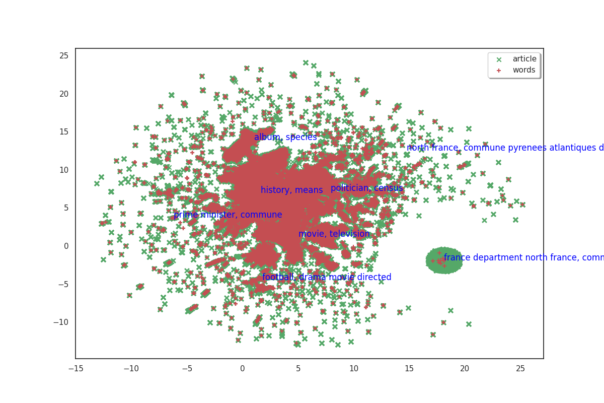
On the plot above, articles are shown in green and words in red. Because we don’t have labels for the points, it doesn’t make much sense as is. But we can see that the data shows some clusters which we could try to identify.
Clustering
In order to identify clusters, we use the KMeans clustering technique on the articles. We’ll also try to label these clusters by selecting the most frequent words that appear in each cluster’s articles.
from cartodata.clustering import create_kmeans_clusters  # noqa

cluster_labels = []
c_lda, c_umap, c_scores, c_knn, _, _, _ = create_kmeans_clusters(8,  # number of clusters to create
                                                        # 2D matrix of articles
                                                        umap_matrices[0],
                                                        # the 2D matrix of words
                                                        umap_matrices[1],
                                                        # the articles to words matrix
                                                        words_mat,
                                                        # word scores
                                                        words_scores,
                                                        # a list of initial cluster labels
                                                        cluster_labels,
                                                        # LDA space matrix of words
                                                        lsa_matrices[1])
c_scores

""
fig, ax = plot(umap_matrices)

for i in range(8):
    ax.annotate(c_scores.index[i], (c_umap[0, i], c_umap[1, i]),
                color='blue')
Total running time of the script: (23 minutes 19.103 seconds)