Note
Go to the end to download the full example code.
Processing LISN data with Pipeline API (LSA projection)
In this example we will process LISN (Laboratoire Interdisciplinaire des Sciences du Numérique) dataset using Pipeline API. LISN dataset contains all articles from HAL (https://hal.archives-ouvertes.fr/) published by authors from LISN between 2000-2022.
The pipeline will comprise of the following steps:
extract entities (articles, authors, teams, labs, words) from a collection of scientific articles
use Latent Semantic Analysis (LSA) to generate n-dimensional vector representation of the entities
use Uniform Manifold Approximation and Projection (UMAP) to project those entities in 2 dimensions
use HDBScan clustering to cluster entities
find their nearest neighbors.
Create LISN Dataset
We will first create Dataset for LISN.
The CSV file containing the data can be downloaded from https://zenodo.org/record/7323538/files/lisn_2000_2022.csv . We will use version 2.0.0 of the dataset. When we specify the URL to CSVDataset, it will download the file if it does not exist locally.
from cartodata.pipeline.datasets import CSVDataset  # noqa
from pathlib import Path # noqa

ROOT_DIR = Path.cwd().parent
# The directory where files necessary to load dataset columns reside
INPUT_DIR = ROOT_DIR / "datas"
# The directory where the generated dump files will be saved
TOP_DIR = ROOT_DIR / "dumps"

dataset = CSVDataset(name="lisn", input_dir=INPUT_DIR, version="2.0.0", filename="lisn_2000_2022.csv",
                       fileurl="https://zenodo.org/record/7323538/files/lisn_2000_2022.csv",
                       columns=None, index_col=0, top_dir=TOP_DIR)
This will check if the dataset file already exists locally. If it does not, it downloads the file from the specified URL and the loads the file to a pandas Dataframe.
Let’s view the dataset.
df = dataset.df

df.head(5)
Downloading data from https://zenodo.org/records/7323538/files/lisn_2000_2022.csv (6.3 MB)


file_sizes:   0%|                                   | 0.00/6.59M [00:00<?, ?B/s]
file_sizes:  51%|█████████████▎            | 3.37M/6.59M [00:00<00:00, 33.3MB/s]
file_sizes: 100%|██████████████████████████| 6.59M/6.59M [00:00<00:00, 44.1MB/s]
Successfully downloaded file to /builds/2mk6rsew/0/hgozukan/cartolabe-data/dumps/lisn/2.0.0/lisn_2000_2022.csv
The dataframe that we just read consists of 4262 articles as rows.
df.shape[0]
4262
And their authors, abstract, keywords, title, research labs and domain as columns.
print(*df.columns, sep="\n")
structId_i
authFullName_s
en_abstract_s
en_keyword_s
en_title_s
structAcronym_s
producedDateY_i
producedDateM_i
halId_s
docid
en_domainAllCodeLabel_fs
Now we should define our entities and set the column names corresponding to those entities from the data file. We have 5 entities:
———|-------------| | articles | en_title_s | | authors | authFullName_s | | teams | structAcronym_s | | labs | structAcronym_s | | words | en_abstract_s, en_title_s, en_keyword_s, en_domainAllCodeLabel_fs |
Cartolabe provides 4 types of columns:
IdentityColumn: The entity of this column represents the main entity of the dataset. The column data corresponding to the entity in the file should contain a single value and this value should be unique among column values. There can only be one IdentityColumn in the dataset.
CSColumn: The entity of this column type is related to the main entity, and can contain single or comma separated values.
CorpusColumn: The entity of this column type is the corpus related to the main entity. This can be a combination of multiple columns in the file. It uses a modified version of CountVectorizer(https://scikit-learn.org/stable/modules/generated/sklearn.feature_extraction.text.CountVectorizer.html#sklearn.feature_extraction.text.CountVectorizer).
TfidfCorpusColumn: The entity of this column type is the corpus related to the main entity. This can be a combination of multiple columns in the file or can contain filepath from which to read the text corpus. It uses TfidfVectorizer (https://scikit-learn.org/stable/modules/generated/sklearn.feature_extraction.text.TfidfVectorizer.html).
In this dataset, Articles is our main entity. We will define it as IdentityColumn:
from cartodata.pipeline.columns import IdentityColumn, CSColumn, CorpusColumn  # noqa

articles_column = IdentityColumn(nature="articles", column_name="en_title_s")
authFullName_s column for entity authors in the dataset lists the authors who have authored each article, and has comma separated values. We will define a CSColumn:
authors_column = CSColumn(nature="authors", column_name="authFullName_s", filter_min_score=4)
Here we have set filter_min_score=4 to indicate that, while processing data, authors who have authored less than 4 articles will be filtered. When it is not set, the default value is 0, meaning that entities will not be filtered.
Teams and Labs entities both use structAcronym_s column which also has comma separated values. structAcronym_s column contains both teams and labs of the articles. For teams entity we will take only teams and for labs entity we will take only labs.
The file ../datas/inria-teams.csv contains the list of Inria teams. For teams entity, we will whitelist the values from inria-teams.csv and for labs entity, we will blacklist values from inria-teams.csv.
teams_column = CSColumn(nature="teams", column_name="structAcronym_s", whitelist="inria-teams.csv",
                        filter_min_score=4)

labs_column = CSColumn(nature="labs", column_name="structAcronym_s", blacklist="inria-teams.csv",
                        filter_min_score=4)
For words entity, we are going to use multiple columns to create a text corpus for each article:
words_column = CorpusColumn(nature="words",
                            column_names=["en_abstract_s", "en_title_s", "en_keyword_s", "en_domainAllCodeLabel_fs"],
                            stopwords="stopwords.txt", nb_grams=4, min_df=10, max_df=0.05,
                            min_word_length=5, normalize=True)
Now we are going to set the columns of the dataset:
dataset.set_columns([articles_column, authors_column, teams_column, labs_column, words_column])
We can set the columns in any order that we prefer. We will set the first entity as identity entity and the last entity as the corpus. If we set the entities in a different order, the Dataset will put the main entity as first.
The dataset for LISN data is ready. Now we will create and run our pipeline. For this pipeline, we will:
run LSA projection -> N-dimesional
run UMAP projection -> 2D
cluster entities
find nearest neighbors
Create and run pipeline
We will first create a pipeline with the dataset. We will set hierarchical_dirs=True to save each entity generated in a directory named with the parameters of generation and places in a hierarchy.
from cartodata.pipeline.common import Pipeline  # noqa

pipeline = Pipeline(dataset=dataset, top_dir=TOP_DIR, input_dir=INPUT_DIR, hierarchical_dirs=True)
The workflow generates the natures from dataset columns.
pipeline.natures
['articles', 'authors', 'teams', 'labs', 'words']
Creating correspondance matrices for each entity type
From this table of articles, we want to extract matrices that will map the correspondance between these articles and the entities we want to use.
Pipeline has generate_entity_matrices function to generate matrices and scores for each entity (nature) specified for the dataset.
matrices, scores = pipeline.generate_entity_matrices(force=True)
The order of matrices and scores correspond to the order of dataset columns specified.
dataset.natures
['articles', 'authors', 'teams', 'labs', 'words']
Articles
The first matrix in matrices and Series in scores corresponds to articles.
The type for article column is IdentityColumn. It generates a matrix that simply maps each article to itself.
articles_mat = matrices[0]
articles_mat.shape
(4262, 4262)
Having type IdentityColumn, each article will have score 1.
articles_scores = scores[0]
articles_scores.shape

""
articles_scores.head()
Termination and Confluence of Higher-Order Rewrite Systems                                    1.0
Efficient Self-stabilization                                                                  1.0
Resource-bounded relational reasoning: induction and deduction through stochastic matching    1.0
Reasoning about generalized intervals : Horn representability and tractability                1.0
Proof Nets and Explicit Substitutions                                                         1.0
dtype: float64
Authors
The second matrix in matrices and score in scores correspond to authors.
The type for authors column is CSColumn. It generates a sparce matrix where rows correspond to articles and columns corresponds to authors.
authors_mat = matrices[1]
authors_mat.shape
(4262, 694)
Here we see that after filtering authors which have less than 4 articles, there are 694 distinct authors.
The series, which we named authors_scores, contains the list of authors extracted from the column authFullName_s with a score that is equal to the number of rows (articles) that this value was mapped within the authors_mat matrix.
authors_scores = scores[1]
authors_scores.head()
Sébastien Tixeuil       47
Michèle Sebag          137
Khaldoun Al Agha        20
Ralf Treinen             5
Christine Eisenbeis     27
dtype: int64
If we look at the 4th column of the matrix, which corresponds to the author Ralf Treinen, we can see that it has 5 non-zero rows, each row indicating which articles he authored.
print(authors_mat[:, 3])
(6, 0)        1
(21, 0)       1
(37, 0)       1
(2729, 0)     1
(3573, 0)     1
Teams
The third matrix in matrices and score in scores correspond to teams.
The type for teams column is CSColumn. It generates a sparce matrix where rows correspond to articles and columns corresponds to teams.
teams_mat = matrices[2]
teams_mat.shape
(4262, 33)
Here we see that after filtering teams which have less than 4 articles, there are 33 distinct teams.
The series, which we named teams_scores, contains the list of teams extracted from the column structAcronym_s with a score that is equal to the number of rows (articles) that this value was mapped within the teams_mat matrix.
teams_scores = scores[2]
teams_scores.head()
TAO        533
Regal       10
Parkas      14
DAHU         7
GALLIUM     23
dtype: int64
Labs
The fourth matrix in matrices and score in scores correspond to labs.
The type for labs column is CSColumn. It generates a sparce matrix where rows correspond to articles and columns corresponds to labs.
labs_mat = matrices[3]
labs_mat.shape
(4262, 549)
Here we see that after filtering labs which have less than 4 articles, there are 549 distinct labs.
The series, which we named labs_scores, contains the list of labs extracted from the column structAcronym_s with a score that is equal to the number of rows (articles) that this value was mapped within the labs_mat matrix.
labs_scores = scores[3]
labs_scores.head()
LRI      4789
UP11     6271
CNRS    10217
LISN     5203
X         487
dtype: int64
Words
The fifth matrix in matrices and score in scores correspond to words.
The type for words column is CorpusColumn. It creates a corpus merging multiple text columns in the dataset, and then extracts n-grams from that corpus. Finally it generates a sparce matrix where rows correspond to articles and columns corresponds to n-grams.
words_mat = matrices[4]
words_mat.shape
(4262, 4645)
Here we see that there are 5226 distinct n-grams.
The series, which we named words_scores, contains the list of n-grams with a score that is equal to the number of rows (articles) that this value was mapped within the words_mat matrix.
words_scores = scores[4]
words_scores.head()
abilities     21
ability      164
absence       53
absolute      19
abstract     174
dtype: int64
Dimension reduction
One way to see the matrices that we created is as coordinates in the space of all articles. What we want to do is to reduce the dimension of this space to make it easier to work with and see.
LSA projection
We’ll start by using the LSA (Latent Semantic Analysis) technique to reduce the number of rows in our data.
from cartodata.pipeline.projectionnd import LSAProjection  # noqa

num_dim = 80

lsa_projection = LSAProjection(num_dim)

pipeline.set_projection_nd(lsa_projection)
Now we can run LSA projection on the matrices.
matrices_nD = pipeline.do_projection_nD(force=True)

""
for nature, matrix in zip(pipeline.natures, matrices_nD):
    print(f"{nature}  -------------   {matrix.shape}")
articles  -------------   (80, 4262)
authors  -------------   (80, 694)
teams  -------------   (80, 33)
labs  -------------   (80, 549)
words  -------------   (80, 4645)
We have 80 rows for each entity.
This makes it easier to work with them for clustering or nearest neighbors tasks, but we also want to project them on a 2D space to be able to map them.
UMAP projection
The UMAP (Uniform Manifold Approximation and Projection) is a dimension reduction technique that can be used for visualisation similarly to t-SNE.
We use this algorithm to project our matrices in 2 dimensions.
from cartodata.pipeline.projection2d import UMAPProjection  # noqa


umap_projection = UMAPProjection(n_neighbors=15, min_dist=0.1)

pipeline.set_projection_2d(umap_projection)
Now we can run UMAP projection on the LSA matrices.
matrices_2D = pipeline.do_projection_2D(force=True)
Now that we have 2D coordinates for our points, we can try to plot them to get a feel of the data’s shape.
labels = tuple(pipeline.natures)
colors = ['b', 'r', 'c', 'y', 'm']

fig, ax = pipeline.plot_map(matrices_2D, labels, colors)
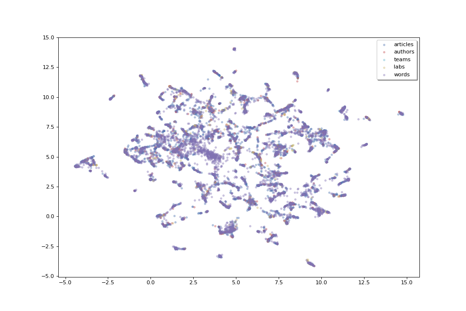
The plot above, as we don’t have labels for the points, doesn’t make much sense as is. But we can see that the data shows some clusters which we could try to identify.
Clustering
In order to identify clusters, we use the HDBScan clustering technique on the articles. We’ll also try to label these clusters by selecting the most frequent words that appear in each cluster’s articles.
from cartodata.pipeline.clustering import HDBSCANClustering  # noqa

# level of clusters, hl: high level, ml: medium level
cluster_natures = ["hl_clusters", "ml_clusters"]

hdbscan_clustering = HDBSCANClustering(n=8, base_factor=3, natures=cluster_natures)

pipeline.set_clustering(hdbscan_clustering)
Now we can run clustering on the matrices.
(clus_nD, clus_2D, clus_scores, cluster_labels,
cluster_eval_pos, cluster_eval_neg) = pipeline.do_clustering()
Nothing in cache, initial Fitting with min_cluster_size=15 Found 98 clusters in 0.2496061189995089s
Max Fitting with min_cluster_size=30 Found 53 clusters in 0.11711032799939858s
Max Fitting with min_cluster_size=60 Found 18 clusters in 0.09962272899974778s
Max Fitting with min_cluster_size=120 Found 11 clusters in 0.08927081399997405s
Max Fitting with min_cluster_size=240 Found 4 clusters in 0.08782700699975976s
Midpoint Fitting with min_cluster_size=180 Found 7 clusters in 0.09113641800013284s
Midpoint Fitting with min_cluster_size=150 Found 8 clusters in 0.09223331199973472s
No need Re-Fitting with min_cluster_size=150
Clusters cached: [4, 7, 8, 11, 18, 53, 98]
Nothing in cache, initial Fitting with min_cluster_size=15 Found 98 clusters in 0.10032779599987407s
Max Fitting with min_cluster_size=30 Found 53 clusters in 0.09995358900050633s
Max Fitting with min_cluster_size=60 Found 18 clusters in 0.098051748999751s
Midpoint Fitting with min_cluster_size=45 Found 28 clusters in 0.09810328700041282s
Midpoint Fitting with min_cluster_size=52 Found 18 clusters in 0.09916086700013693s
Re-Fitting with min_cluster_size=45 Found 28 clusters in 0.09848179599975992s
Clusters cached: [18, 18, 28, 53, 98]
As we have specified two levels of clustering, the returned lists wil have two values.
len(clus_2D)
2
We will now display two levels of clusters in separate plots, we will start with high level clusters:
clus_scores_hl = clus_scores[0]
clus_mat_hl = clus_2D[0]


fig_hl, ax_hl = pipeline.plot_map(matrices_2D, labels, colors,
                                  title="LISN Dataset High Level Clusters",
                                  annotations=clus_scores_hl.index, annotation_mat=clus_mat_hl)
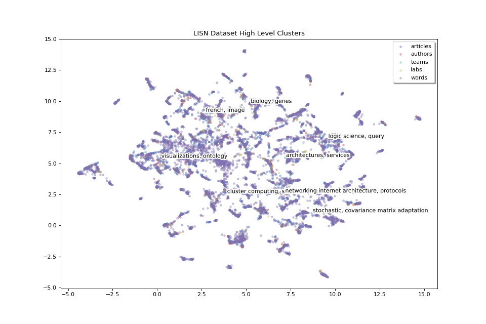
The 8 high level clusters that we created give us a general idea of what the big clusters of data contain.
With medium level clusters we have a finer level of detail:
clus_scores_ml = clus_scores[1]
clus_mat_ml = clus_2D[1]

fig_ml, ax_ml = pipeline.plot_map(matrices_2D, labels, colors,
                                  title="LISN Dataset Medium Level Clusters",
                                  annotations=clus_scores_ml.index, annotation_mat=clus_mat_ml,
                                  annotation_color='black')
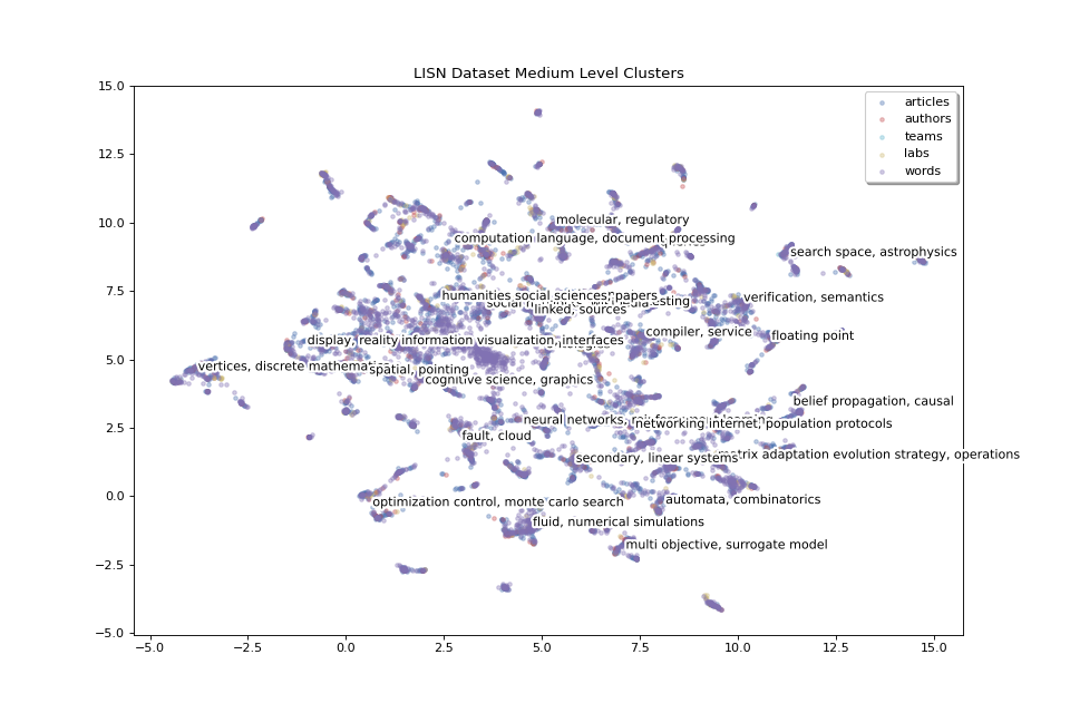
We have 24 medium level clusters. We can increase the number of clusters to have even finer details to zoom in and focus on smaller areas.
Now we will save the plots in the working_dir directory.
pipeline.save_plots()
[(<Figure size 960x640 with 1 Axes>, 'lisn_2.0.0_15d3d1d060e5f28d_lsa_80_True_umap_euclidean_15_0.1_random_1.0_None_None_hdbscan_hl_clusters.png'), (<Figure size 960x640 with 1 Axes>, 'lisn_2.0.0_15d3d1d060e5f28d_lsa_80_True_umap_euclidean_15_0.1_random_1.0_None_None_hdbscan_ml_clusters.png')]
The plots for 2D map is saved under pipeline 2D directory.
for file in pipeline.get_2D_dir().glob("*.png"):
    print(file)
/builds/2mk6rsew/0/hgozukan/cartolabe-data/dumps/lisn/2.0.0/mat_articles__authors_4_teams_4_labs_4_words_en_abstract_s_en_title_s_en_keyword_s_en_domainAllCodeLabel_fs_10_0.05_None_None_5_4/lsa_80_True/umap_euclidean_15_0.1_random_1.0_None_None/lisn_2.0.0_15d3d1d060e5f28d_lsa_80_True_umap_euclidean_15_0.1_random_1.0_None_None.png
The plots for 2D map with clustering is saved under pipeline cluster directory.
for file in pipeline.get_clus_dir().glob("*.png"):
    print(file)
/builds/2mk6rsew/0/hgozukan/cartolabe-data/dumps/lisn/2.0.0/mat_articles__authors_4_teams_4_labs_4_words_en_abstract_s_en_title_s_en_keyword_s_en_domainAllCodeLabel_fs_10_0.05_None_None_5_4/lsa_80_True/umap_euclidean_15_0.1_random_1.0_None_None/hdbscan_3/lisn_2.0.0_15d3d1d060e5f28d_lsa_80_True_umap_euclidean_15_0.1_random_1.0_None_None_hdbscan_hl_clusters.png
/builds/2mk6rsew/0/hgozukan/cartolabe-data/dumps/lisn/2.0.0/mat_articles__authors_4_teams_4_labs_4_words_en_abstract_s_en_title_s_en_keyword_s_en_domainAllCodeLabel_fs_10_0.05_None_None_5_4/lsa_80_True/umap_euclidean_15_0.1_random_1.0_None_None/hdbscan_3/lisn_2.0.0_15d3d1d060e5f28d_lsa_80_True_umap_euclidean_15_0.1_random_1.0_None_None_hdbscan_ml_clusters.png
Nearest neighbors
One more thing which could be useful to appreciate the quality of our data would be to get each point’s nearest neighbors. If our data processing is done correctly, we expect the related articles, labs, words and authors to be located close to each other.
Finding nearest neighbors is a common task with various algorithms aiming to solve it. The find_neighbors method uses one of these algorithms to find the nearest points of all entities (articles, authors, teams, labs, words). It takes an optional weight parameter to tweak the distance calculation to select points that have a higher score but are maybe a bit farther instead of just selecting the closest neighbors.
from cartodata.pipeline.neighbors import AllNeighbors

n_neighbors = 10
weights = [0, 0.5, 0.5, 0, 0]

neighboring = AllNeighbors(n_neighbors=n_neighbors, power_scores=weights)

pipeline.set_neighboring(neighboring)

pipeline.find_neighbors()
Export file using exporter
We can now export the data. To export the data, we need to configure the exporter.
The exported data will be the points extracted from the dataset corresponding to the entities that we have defined.
In the export file, we will have the following columns for each point:
———|-------------| | nature | one of articles, authors, teams, labs, words | | label | point’s label | | score | point’s score | | rank | point’s rank | | x | point’s x location on the map | | y | point’s y location on the map | | nn_articles | neighboring articles to this point | | nn_teams | neighboring teams to this point | | nn_labs | neighboring labs to this point | | nn_words | neighboring words to this point |
we will call pipeline.export function. It will create export.feather file and save under pipeline.working_dir.
pipeline.export()
Let’s display the contents of the file. The file is saved under the pipeline cluster directory.
import pandas as pd # noqa

df = pd.read_feather(pipeline.get_clus_dir() / "export.feather")
df.head()
This is a basic export file. For each point, we can add additional columns.
For example, for each author, we can add labs and teams columns to list the labs and teams that the author belongs to. We can also merge the teams and labs in one column and name it as labs. To do that we have to first create export config for the entity (nature) that we would like to modify.
from cartodata.pipeline.exporting import (
    ExportNature, MetadataColumn
) # noqa

ex_author = ExportNature(key="authors",
                         refs=["labs", "teams"],
                         merge_metadata=[{"columns": ["teams", "labs"],
                                          "as_column": "labs"}])
We can do the same for articles. Each article will have teams and labs data, and additionally author of the article. So we can set refs=[“labs”, “teams”, “authors”].
The original dataset contains a column producedDateY_i which contains the year that the article is published. We can add this data as metadata for the point but updating column name with a more clear alternative year. We can also add a function to apply to the column value. In this example we will convert column value to string.
meta_year_article = MetadataColumn(column="producedDateY_i", as_column="year",
                                   func="x.astype(str)")
We will also add halId_s column as url and set empty string if the value does not exist:
meta_url_article = MetadataColumn(column="halId_s", as_column="url", func="x.fillna('')")

""
ex_article = ExportNature(key="articles", refs=["labs", "teams", "authors"],
                         merge_metadata=[{"columns": ["teams", "labs"],
                                          "as_column": "labs"}],
                         add_metadata=[meta_year_article, meta_url_article])

pipeline.export(export_natures=[ex_article, ex_author])
Now we can load the new export.feather file to see the difference.
df = pd.read_feather(pipeline.get_clus_dir()/ "export.feather")

df.head()
For the points of nature articles, we have additional labs, authors, year, url columns.
Let’s see the points of nature authors:
df[df["nature"] == "authors"].head()
We have values for labs field, but not for authors, year, or url field.
As we have not defined any relation for points of natures teams, labs and words, these new columns are empty for those points.
df[df["nature"] == "teams"].head()

""
df[df["nature"] == "labs"].head()

""
df[df["nature"] == "words"].head()

""
df['x'][1]
7.495028972625732
Hierarchical Directory Structure
It is possible to save the files generated by pipeline in a hierarchical directory structure. The advantage for this is to be able to use the same matrices whenever the parameters are the same, and regenerate new ones, once there is a change of parameters in a particular step. The previous processing will not be deleted, and it will enable us to compare the results of multiple runs on the same dataset with different parameters.
pipeline.working_dir is the top directory that for a processing. It is named with dataset column parameters. The entity matrices and all following processing artifacts are saved under this directory.
pipeline.working_dir
PosixPath('/builds/2mk6rsew/0/hgozukan/cartolabe-data/dumps/lisn/2.0.0/mat_articles__authors_4_teams_4_labs_4_words_en_abstract_s_en_title_s_en_keyword_s_en_domainAllCodeLabel_fs_10_0.05_None_None_5_4')
nD processing dumps are saved under pipeline.working_dir / nD_dir.
pipeline.get_nD_dir()
PosixPath('/builds/2mk6rsew/0/hgozukan/cartolabe-data/dumps/lisn/2.0.0/mat_articles__authors_4_teams_4_labs_4_words_en_abstract_s_en_title_s_en_keyword_s_en_domainAllCodeLabel_fs_10_0.05_None_None_5_4/lsa_80_True')
2D processing dumps are saved under pipeline.working_dir / nD_dir / 2D_dir.
pipeline.get_2D_dir()
PosixPath('/builds/2mk6rsew/0/hgozukan/cartolabe-data/dumps/lisn/2.0.0/mat_articles__authors_4_teams_4_labs_4_words_en_abstract_s_en_title_s_en_keyword_s_en_domainAllCodeLabel_fs_10_0.05_None_None_5_4/lsa_80_True/umap_euclidean_15_0.1_random_1.0_None_None')
Clustering dumps are saved under pipeline.working_dir / nD_dir / 2D_dir/ clus_dir.
pipeline.get_clus_dir()
PosixPath('/builds/2mk6rsew/0/hgozukan/cartolabe-data/dumps/lisn/2.0.0/mat_articles__authors_4_teams_4_labs_4_words_en_abstract_s_en_title_s_en_keyword_s_en_domainAllCodeLabel_fs_10_0.05_None_None_5_4/lsa_80_True/umap_euclidean_15_0.1_random_1.0_None_None/hdbscan_3')
Neighboring dumps are saved under pipeline.working_dir / nD_dir / 2D_dir/ neigbors_dir.
pipeline.get_neighbors_dir()
PosixPath('/builds/2mk6rsew/0/hgozukan/cartolabe-data/dumps/lisn/2.0.0/mat_articles__authors_4_teams_4_labs_4_words_en_abstract_s_en_title_s_en_keyword_s_en_domainAllCodeLabel_fs_10_0.05_None_None_5_4/lsa_80_True/neighbors_10_0_0.5_0.5_0_0')
Let’s assume that we want to run UMAP with different parameters.
from cartodata.pipeline.projection2d import UMAPProjection  # noqa


umap_projection = UMAPProjection(n_neighbors=30, min_dist=0.3)

pipeline.set_projection_2d(umap_projection)
matrices_2D = pipeline.do_projection_2D()
labels = tuple(pipeline.natures)
colors = ['b', 'r', 'c', 'y', 'm']

fig, ax = pipeline.plot_map(matrices_2D, labels, colors)

If we list the contents of nD directory, we will see two directories for umap projection.
dir_nD = pipeline.get_nD_dir()

""
# !ls $dir_nD
''
Total running time of the script: (0 minutes 47.179 seconds)